A New View on Migration Processes between SIR Centra An Account of the Different Dynamics of Host and Guest
*Corresponding Author(s):
Igor SazonovSwansea University, Singleton Park, SA2 8PP, United Kingdom
Tel:+44 1792602767,
Email:i.sazonov@swansea.ac.uk
Abstract
We study an epidemic propagation between M population centra. The novelty of the model lies in the explicit analysis of the dynamics of host (remaining in the same centre) and guest (migrated to another centre) populations separately. Even in the simplest case M = 2, this modification is justified because it gives a more realistic description of migration processes. Standard migration terms in coupled SIR models can show a very unrealistic instability in total population size, as can be demonstrated simply by removing infection parameters. It is also important to account for a certain number of guest susceptibles present in non-host centra because these susceptibles may be infected and return to the host node as infectives. This effect can be non-trivial. Although the relative numbers of these guests will be low, their contribution to the epidemic process may not be assumed to be negligible, because the return rate of a guest individual will, by nature, tend to be high. That is, the trigger of an outbreak in a new center may often be caused by an original member of the centre returning (infected) from a visit to an infected center, and not just by migration movements of (infected) individuals that usually belong in the source centre. In the former case the number of infected is low but the migration rate high, in the latter, vice versa. Therefore both processes may contribute significantly to the dynamics. In addition to providing a more appropriate model for migration processes, we show that taking account the flux of both host and guest infectives noticeably increases the speed of epidemic spread in a 1D lattice of identical SIR centra, and we explore how the dynamics are dependent on the rates of the migration processes and the relative centre population sizes.
Keywords
INTRODUCTION
The classical SIR model is one of the cornerstones of mathematical epidemiology. In this model, the population is assumed to consist of three components: susceptibles S, infectives I and removeds R (recovered or dead) satisfying the following ODEs [1-3].
 (1)
(1)
Where α and β are respectively recovering and contamination rates; and dot denotes the time derivative. This model describes a typical directly transmitted disease (rather than vector borne) outbreak in a populated center: the contamination stage, the developing outbreak with a peak, and the epidemic fadeout after the peak. The classical SIR model remains the building block for many, more complicated applied epidemic models.
Models of coupled epidemic centra are of particular interest because they describe epidemic spread through network of populated centra, and hence the overall population is not treated as a homogenous system. Within a center, or node in the network, the outbreak might be described by an SIR-type model, but the links between nodes then describe how the disease might spread between centers. This is a subject of intensive research [4-8] and relates now, not just to disease spread from neighboring towns or cities, but to rapid propagation around the globe [9,10]. These models have led to insights into the epidemic processes in linked centra. For example, it was observed that on heterogeneous networks, an increase in the movement of population may decrease the size of the epidemic at the steady state, but it increases the chances of outbreak. This was the motivation for this detailed exploration of the migration processes in heterogeneous populations.
The coupling between nodes of such a network is mainly caused by migration processes of infectives. There are several models describing such coupling [2,3], for example in [11] the influence of various parameters on the spatial and temporal spread of the disease is studied numerically, with particular focus on the role of quarantine in the form of travel restrictions. In [12,13], the so-called diffusion like model is proposed and studied in the framework of a fast migration time approximation. Note that the model in [11] is a particular case of the diffusion model when the migration time tends to infinity but the coupling coefficient introduced in [12] tends to zero.
In all these models the guest population is completely mixed with the host one, so their dynamics are indistinguishable. Nevertheless, a more detailed consideration suggests that while the epidemic dynamics might be the same, the migration dynamics should be different, especially if considered as part of a discrete randomized model approach which is important at the start of an outbreak, and therefore by definition should be considered in the ‘sparking’ of new outbreaks due to movement of infectives [14-16].
In the paper we start with consideration of the simplest network of only two interacting epidemic SIR centra and study in detail the migration processes and their influence on the population dynamics. Moreover, our interest in the model is motivated by the fact that it serves as a hydrodynamic approximation of a natural Markov process describing the stochastic dynamics of the system [17]. This topic will be explored more fully in a subsequent paper.
To examine the migration model we first consider here the case when epidemic parameters are temporally switched off. The study of migration in isolation provides a simple tractable model and allows us to specify the parameters in a consistent way. Equally important, this analysis reveals that many models used in the literature are unstable in the limit of vanishing infection [3,18]. Other ones remain stable but lead to non-realistic results [19,20].
A suitable approximation is required to avoid numerical integration and to obtain practical formulas for outbreak time, fadeout time and other parameters. In our previous works, we introduced the ‘Small Initial Contagion’ (SIC) approximation, based on the assumption that an outbreak in every population center is caused by relatively small number of initially infectives [12,13,15]. This approximation is appropriate when the model is applied to strongly populated centra like urban centra (i.e., in the situation when the reaction-diffusion model is not accurate).
In the paper we also show how the model can be generalized on the general network of epidemic centra. As an example, a characteristic equation for the travelling wave in a chain of the population centers is derived and its numerical solution is plotted and analyzed.
The paper is organized as follows. In section 4 we derive the equation governing the epidemic and migration dynamics between two SIR centra. In section 5 we isolate the migration process by ‘switching off’ temporally the epidemic dynamics and show that the proposed migration model satisfies intuitive requirements. In section 6 we examine the traditional pure migration models and show that they do not satisfy some reasonable requirements. In section 7 numerical examples of outbreak dynamics are presented. In section 8 we derive a simplified equation in the SIC approximation and estimate the outbreak time in the epidemic centra. In section 9 we consider a more general network and examine epidemic travelling wave in a 1D lattice of coupled epidemic centra as an example.
GOVERNING EQUATIONS
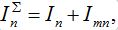
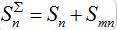
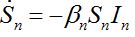
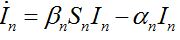
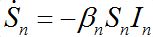
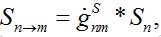
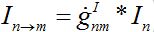
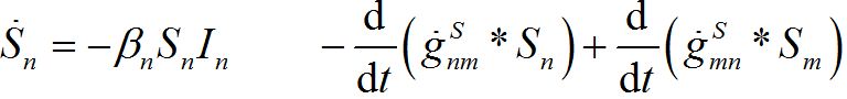
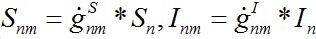
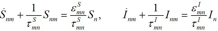
Consider two populated nodes, 1 and 2, with populations N1 and N2, respectively. Let Sn(t), In(t), Rn(t) be the numbers of host susceptibles, infectives and removed, respectively, in node n at time t. Let Smn(t), Imn(t), Rmn(t) be numbers of guest susceptibles, infectives and removed, respectively, in node n migrated from node m at time t. Removed populations Rn, Rnm do not affect dynamics of all others in the framework of the standard SIR model, and we omit them from consideration here. Then, two SIR centers (nodes) interacting due to the migration of individuals between them is described by the following model: the dynamics of hosts in node n obeys the ODEs
 (2)
(2)
 (3)
(3)
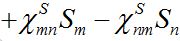
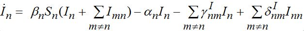
Where n = 1,2; m = 2,1. Here the term βnSn(In+Imn) appears due to infectives Imn migrated from node m and contributing to the total disease transmission process. Terms  and
and  describe migration fluxes (rates) from node n to node m for susceptibles and infectives, respectively. Terms and describe return migration fluxes (rates) to node n for guest individuals in node m. We specify these below.
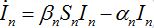
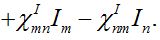
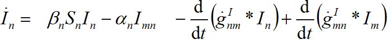
The dynamics of guests in node n temporally arriving from node m can be described by analogous ODEs
 (4)
(4)
 (5)
(5)
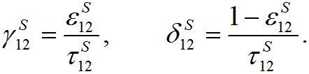
We assume the migration rate is proportional to the population size in the node from which they emigrate. So, we approximate the fluxes as
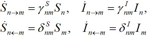 (6)
(6)
where γ’s and δ’s are the forward and backward migration coefficients, respectively.
Our interest in the dynamical equations presented above is motivated by the fact that they serve as a hydrodynamic approximation of a Markov process model. In this context, γ’s can be associated with the transition rate for a host individual to migrate to another node in a unit of time, and δ’s with the transition rate for a guest individual to return to the host node.
Clearly, average return rates should be higher: γnmS < δnmS; γ nmI δInm, otherwise an individual would spend most of the time out of the home center.
Substituting (6) into (2)-(3) and (4)-(5) yields a closed system of ODEs: for the hosts in node n
 (7)
(7)
 (8)
(8)
and for the guests migrated from node m into node n
 (9)
(9)
 (10)
(10)
Evidently, the dynamics of hosts and guests are different.
Typical initial conditions for epidemiological problem describe a number of infectives, say I01; that appeared at t=0 in node 1 only:
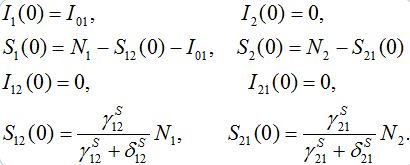 (11)
(11)
The choice for values for S12(0) and S21(0) will be explained below in section 5 by considering that the migration processes reach steady state before the epidemic starts.
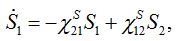
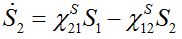
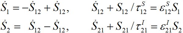
PURE MIGRATION
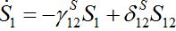 (12)
(12)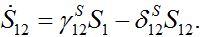 (13)
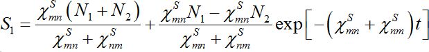
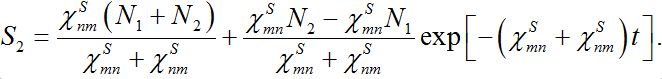
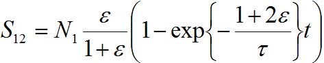
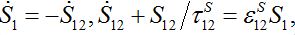
(13)Let migration start at t=0 with the initial conditions S1(0)=N1, S12(0)=0. The solution to such an initial value problem is
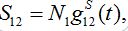
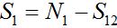 (14)
(14)Where,
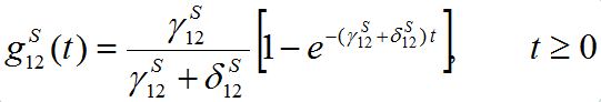 (15)
(15)is the response function (see below). Similar formulas are valid for the second pair: S2; S21. Thus, the number of migrants exponentially tends to some limiting values
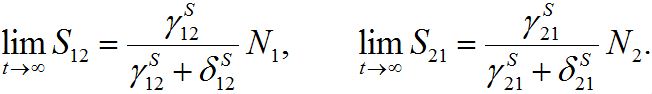 (16)
(16)These limits represent the dynamic equilibrium of migration processes in the absence of the outbreak. At the equilibrium, the forward and backward migrations fluxes compensate each other:
So, in virtue of (6),
Substituting S1=N1-S12 and resolving with respect to S12 yields (16). We take the equilibrium values from (16) as the initial conditions for the outbreak problem that is reflected in (11).
The total populations in any node
 and
and  are described as
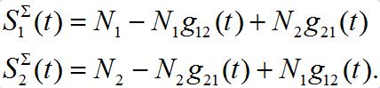
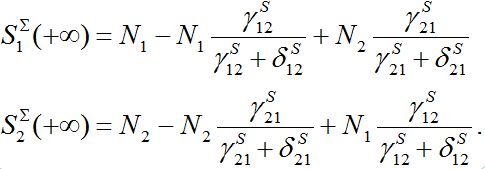
They can be non-monotonic for some choice of parameters. Next,
 asymptotically converges to
If both centra are identical then their total population remains constant.
The migration dynamics described by this model seems reasonable. The migration process resembles a diffusion process in physics, in which the concentration tends monotonically to equilibrium.
Note that, if
 then
then 
i.e., only a small share of the population from node 1 is currently in node 2 and similarly: if
 then
then 
which is appropriate for large population centra. So, in this approximation
To understand why function (15) can be associated with a response function, consider a model for which the number of susceptibles can vary even in the absence of migration due to other reasons (e.g., birth and death). Let
 be the rate of incoming (
 ) or outgoing (
 ) individuals, i.e., the external source in the equations
 (17)
(17)with initial conditions S1(0)=N01; S12(0)=0. Integrating the second equation in view of relation S1=N1-S12yields:

where the asterisk denotes the convolution,
 is the derivative of function (15): recall that
where H(t) is the unit-step heaviside function. So,
is the response in the number of guests in node 2 on the population variation in node 1.
and susceptibles
in node n. To compare these models take the sum of eqs. (7), (8) and obtain the equations
 (18)
(18) (19)
(19)Thus, we cannot obtain equations for total numbers of species only: they become coupled with the equations for guest individuals. This complicates the model but makes it more realistic.
Many authors simply insert terms proportional to the relevant population size in neighboring nodes to provide coupling between SIR centra:
 (20)
(20)
 (21)
(21)Where
 are coupling coefficients [3,18]. In the case of pure migration between two centra (αn=βn=0, In=0) they are reduced to
 (22)
(22)Note that this model does not guarantee preservation of the total population size because the sum S1+S2is variable
which is unrealistic, by eliminating one variable we see that the system has unstable dynamics

i.e., a growing particular solution. Thus, the traditional approach does not describe the migration between centra properly. Although this instability can potentially be hidden in the background of the outbreak and not be observable in certain epidemic model scenarios.
Nevertheless, the model can be easily corrected by introducing inverse fluxes [19,20].
 (23)
(23)
 (24)
(24)Then for a pure migration model we have
 (25)
(25)implying S1+S2=const. The solutions of ODEs (25) with initial conditions S1(0)=N1, S2(0)=N2 demonstrate exponential, diffusion like behavior of each node population
 (25)
(25)In the case
 the both solutions tend to
 (25)
(25)i.e., their populations become equal (fully mixed). Thus the dynamics of the corrected model seems to be more realistic but nevertheless does not satisfy an intuitive interpretation of the equilibrium of the migration process that only a small share of guests can be simultaneously in every node rather than a half of the population.
Notice that equations (18)-(19) for the total population size coincide with (23)-(23) if
 and
and  i.e., model (18)-(19) corresponds to the case when the forward and backward migration coefficients are the same that provides the full mixing of the populations of two neighbor centra. Thus model (18)-(19) can be treated as a particular case of the proposed model, but under the conditions of maximal possible coupling.
In [13], in order to obtain more realistic migration dynamics, different flux terms are added to equations (7)-(8) in the form of convolutions (transition terms)
where g’s are the relevant response functions. Then, the dynamics are described by integro-differential equations
 (26)
(26) (27)
(27) (28)
(28)
 (29)
(29) (30)
(30) (31)
(31)For a pure migration model (neglecting the outbreak dynamics) we obtain the following ODEs
 (32)
(32)Taking the sum of the latter equations we see that the total population is preserved: S1+S2=const=N1+N2.
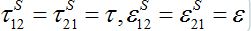
In the case of identical migration parameters for the both nodes:
the number of migrants in node 2 is described as in (14)-(15):
In the general case, the solution can be represented via two exponential functions with different characteristic times τ1 and τ2 and not necessarily monotonic (which is quite unrealistic). Nevertheless, neglecting backward migration from node 2 to node 1 by setting S21=0, i.e., solving equations
yields exactly the solution (14)-(15):

summing up, we conclude that the model proposed in the present work behaves appropriately: at first populations increase exponentially, then they tend monotonically to their final values, say
Other useful approximations will be applied in specific situations.
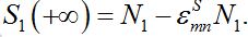
Next we compare the response function (28) defined in [12,13] and the response function (15), and express the basic migration parameters such as the migration characteristic time
 and the coupling coefficient
  via the migration parameters
  and
and  introduced here:
 (33)
(33)The inverse relations are
 (34)
(34)Coefficient
 represents a share of the population from node 1 migrated to node 2 at dynamical equilibrium or a share of time the individuals from node 1 spend in node 2 on average. In the case of relatively small coupling, the estimation of the order of different terms is very useful.
Analogous response functions can be defined for all other population classes. They determine the dynamics due to pure migration when the disease transmission and removal is disregarded by setting α’s and β’s to zero. The response function for the migration of susceptibles and infectives
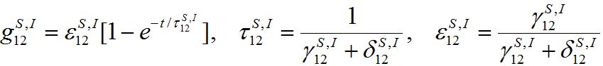 (35)
(35)will be used intensively below.
Thus in contrast to many earlier coupling models used in epidemiology and ecology, the pro-posed migration model depends on two parameters γ, δ or ?, τ. The pairs of parameters are closely related to each other through (33) or (34). For a specific scenario, the migration parameters ?‘s and τ’s can be estimated in advance of an epidemic from demographic data.
NUMERICAL EXAMPLES
Examples of numerical integration of equations (7)-(10) subjected to initial conditions (11) are presented in figures 1 and 2. Here the total share of infectives in every node: 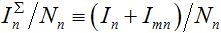 are plotted by the grey line in node 1 and by the colored solid lines in node 2.
Parameters of the basic model are selected as: N1=N2, I01=N1=0:01, ρ1=ρ2=3, α1=α2=1,  Here ρn are the basic reproduction numbers for the nodes n defined for the classical SIR model as [2,3]
(35)
in the assumption that  Next, parameter values in the basic model are modified and the subsequent influence on the epidemic dynamics is examined.
In figure 1, the influence of the basic reproduction number (left) and node populations (right) are shown. Note that the dynamics in node 2 are remarkably different from the standard SIR dynamics when the population ratio is N2/N1=10. Also note that the shoulder in figure 1 (right) for the case of a larger population in node 2 shows the influence of the coupling and the importance of considering the contamination stage. It cannot be produced by a set of single SIR models. In figure 2 one can observe the dependence of the outbreak on the migration parameters: the coupling parameter ? (left) and the characteristic migration time τ (right). Also, we can see that the outbreak in node 1 can be significantly higher than that predicted by the single SIR model if the migration process is included and if the population size is greater in node 2.Note that, when the dynamics of host and guest individuals are treated separately, two migration fluxes are essential in spreading the disease from node to node. Let node 1 is the first to be contaminated.
- Host infectives in node 1 can migrate to node 2(I1 →I1;2) and contaminate susceptibles there (S2 →I2).
Guest susceptibles S21 in node 1 migrated from node 2 can be contaminated in node 1, (S21 →I21) then return to node 2 and start contamination back in their home node.
To show the influence of the second flux on the outbreak dynamics, equations (7)-(10) are integrated, with the initial conditions having S21(0)=0, i.e., when the second flux is neglected, when no guest susceptibles in node 1 can be contaminated and return to node 1. The results of integration are shown by colored dashed lines:  vs t.
vs t.
The colored dotted lines indicate the results obtained using the SIC approximation described in section 8.
SMALL INITIAL CONTAGION (SIC) APPROXIMATION
- Large populations in every center: Nn ? 1;
 (37)
(37) - The migration fluxes between the centers are small:
 (38)
(38) - The initial number of infectives in the first contaminated center, say, n=1, is small: I01 ? N1 (39)
- Contaminating stage: The number of infectives is small
 ,
,  and the fluxes of infectives caused by migration are essential for the outbreak process (except the first node).
 - Developed outbreak: In = O (Nn), when the contribution of migration fluxes is negligible.
- Recovery stage: The node is not affected by infective immigrants and has a slight affect on the contamination of other nodes.
Thus, using the SIC approach, equations (7)-(10) can be significantly simplified at different stages of the outbreak.
To build the asymptotic theory, we assume that all coupling coefficients are of the same order with respect to a small parameter

Also we assume that
Also at contamination stage I2 < O(1) I21,12, S2 ≈ N2 - S21. We rewrite equation (7)-(8) for the host population in node 1 separating O(?) terms and enclosing them in curly brackets
 (40)
(40) (41)
(41)Neglecting terms in curly brackets we see that outbreak in node 1 can be described by the standard SIR model for an isolated node coinciding with (1). This means that the node contaminated first outside the network is insensitive to the outbreak in the second node, which occurs after a certain delay.
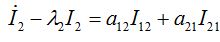
Now we rewrite equation (7)-(8) for the host population in node 2:
 (42)
(42) (43)
(43)Here the terms that remain small and can be neglected are enclosed in curly brackets. Small terms which can prevail at the stage of contamination when I2 is small are enclosed in square brackets.
They are the coupling terms, and represent two fluxes: ν1(t) = β2S2I12 and
 . Flux ν1 is due to the infected individuals belonging to node 1 and currently visiting node 2 thereby spreading infection to susceptibles there. Flux ν2 is due to susceptible individuals visiting node 1 from node 2, becoming infected there, and then returning as infectives to their home node 2.
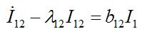
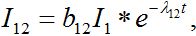
Rewriting equation (10) for I12:
 (44)
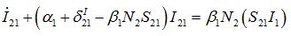
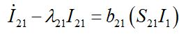
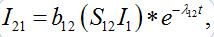
(44)Terms in curly brackets are small and can be neglected. Now we rewrite analogous equation for I21
 (45)
(45)We can neglect terms in curly brackets but the essential term in the square brackets should remain.
The equations (40)-(45) with neglected terms in curly brackets are the ODEs under the SIC approximations. Results of numerical integration of these equations are indicated by colored dotted lines in figures 1 and 2. Comparing the solid and dotted lines these figures, we see that the SIC approximation accurately describes the dynamics in the second node. From figure 2 (left) we conclude that the smaller the coupling parameter ?- the higher the accuracy of the approximation.
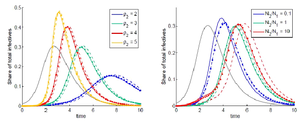
Figure 1: Dynamics of the total share of infectives are indicated by solid lines: grey for node 1 and colored for node 2 for different basic reproduction number ρ1 (left) and different populations (right). Dashed colored lines are obtained by neglecting the initial guest susceptibles in node 1. Dotted line are obtained using the SIC approximation.
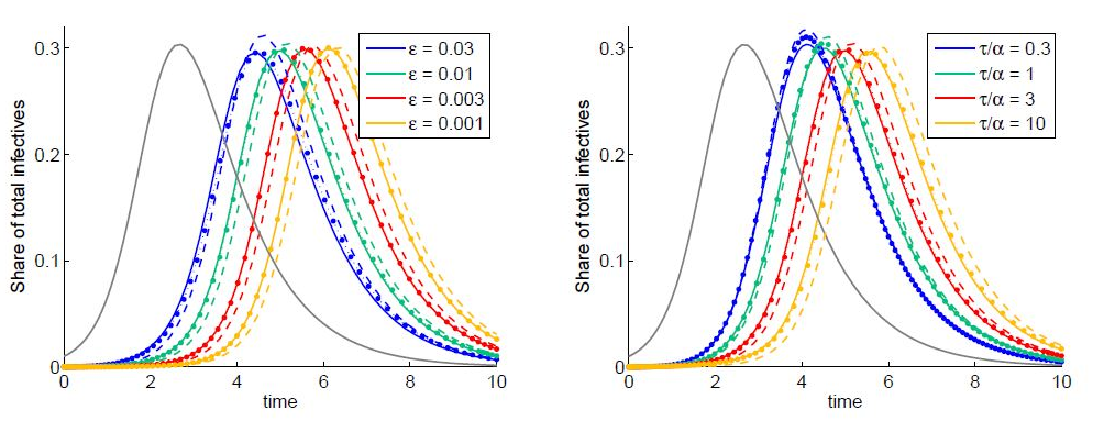
Figure 2: Dynamics of the total share of infectives are indicated by solid lines: grey for node 1 and colored for node 2 for different coupling coefficient ? (left) and migration characteristic time (right). Dashed colored lines are obtained by neglecting the initial guest susceptibles in node 1. Dotted line are obtained using the SIC approximation.
 but can vary during contamination stage. Its dynamics are described by equation (9),
 (46)
(46)It can vary noticeably during the contamination stage for node 2. Neglecting the term in the curly brackets and approximating at this stage S2 ≈ N2 - S21 we obtain the following equation after simple manipulations:
 (47)
(47)Re-writing (40) in the form
 and also utilizing (33) we can write (47) as
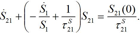 (47)
(47)where S21(0) =
 . When S1=const there is a steady state solution S21=S21(0). In the case of the outbreak the solution can be written in quadrature form
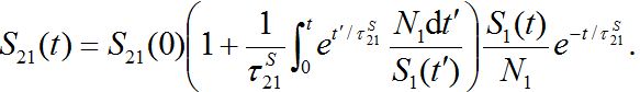 (47)
(47)Coupling with node 1 is essential in the SIC approximation at the initial stage but only before the developed outbreak. At this stage we solve (43)-(46) neglecting terms in the curly brackets (then it becomes a linear inhomogeneous system of ODEs) approximating S2 ≈ N2:
 (48)
(48) (49)
(49) (50)
(50) (51)
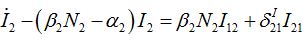
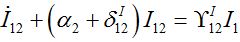
(51)We rewrite first three equations in the simplest form introducing new parameters
 (52)
(52) (53)
(53) (54)
(54)where λ2 = β2N2 - α2 is initial growth rate in node 2;
 and
and  are initial decay rates of guest species I21 and I21, respectively; α12 = β2N2,
  ,Note in the SIC approximation should
  therefore
Solving system (52)-(54) by the Laplace transform method we obtain
 (55)
(55)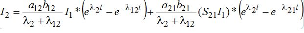 (56)
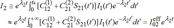
(56)where *denotes the convolution. At time
 only the growing terms for I2 are essential, and the simplified expression takes the form
 (57)
(57)where
 (58)
(58)Constant
 as it is proportional to
  .Constant
  ) is not small but the integrand contains value S21 which is proportional to
  , i.e., also has order O(?).
As I1(t) in the integrand describes an outbreak in node 1 which is a decaying function after reaching the maximal outbreak in the node, we see that contribution of it in integral (57) is negligible after time t* : tb1< t*. Thus for t < t* function I2(t) grows exponentially as in the standard SIR model
 (59)
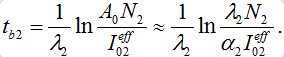
(59)Thus, we have the following evaluation for the effective number of infectives in node 2:
 (60)
(60)The effective number is the initial number of infective I2(0) in an node 2 (considered as an isolated centre) which would give the same outbreak dynamics and the same outbreak time if it was coupled with node 1. This value allows us to estimate the outbreak time tb2 in node 2 in the framework of the SIC approximation. This is illustrated in figure 3.
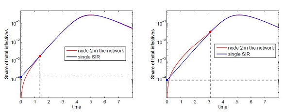
To evaluate the outbreak time, we start with the fact that the development of an outbreak at the first contaminated node is approximately exponential (if the initial share of infective is small):
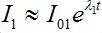 (61)
(61)where ?λ1 is the initial growth rate of infectives in node 1
λ1 = β1S1(0) - α1 ≈ β1N1 – α1 = (ρ1 - 1) (62)
Remind that ρn = βnNn/αn is the basic reproduction number for node n. Subsequent behavior in the first center can be approximated by the limiting solution ilim (t; ρ ) introduced and described in [12,13]
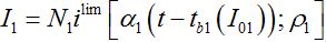 (63)
(63)where, i = I/N is the share of infectives in the node.
The outbreak time tb1(I01) can be roughly approximated by [12,13]
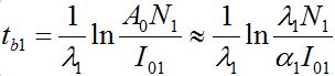 (64)
(64)Where, A0( ρ1) is the parameter of the large negative time asymptotic of the limiting solution:
This shows the share of infectives at the instant of contamination that is required to trigger an outbreak under the assumption that the initial exponential growth continues up to the moment of the peak of the outbreak.
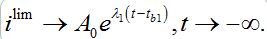
The dynamics of I2 are described by (57) at the initial stages before the developed outbreak: at the contamination stage when the migration of infectives from node 1 is essential and at the stage of exponential growth. At this stage (59) the coupling can be neglected and the dynamics are described by a limiting solution
 (65)
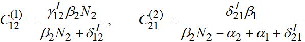
(65)Comparing (59) and (65) we elaborate that
 (66)
(66) (67)
(67) (68)
(68) (69)
(69)Interaction between nodes is determined by M X M matrices
 ,
,  and also matrices of guest populations Smn and Imn. All these matrices have zero diagonal elements, and they may also have zero elements if nodes m and n do not interact directly.
The effective number of initial infectives for the network in the SIC approximation can be calculated by the sum
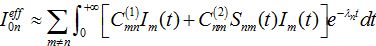 (70)
(70)
It is well known in physics, that far from the source, a cylindrical or spherical wave can be locally approximated by a plane wave, i.e., by a one-dimensional object. So, the similar wave patterns are expected in a grid of interacting centra as in the one dimensional case. Intuitively, consider the 2 dimensional situation of a circular front radiating out from an infected node. As distance from the node increases, the radius increases hence the curvature of the front will tend to be small in comparison with its ‘width’ when it reaches a destination node. Hence the process at that node could have been approximated by a one dimensional travelling wave. We note, however, that this approximation would not necessarily hold for heterogeneous systems, and this will be the attention of future work.
Consider, for example, an infinite 1D lattice of SIR centra where every node n interacts with its nearest neighbors m = n-1 and m = n+1.
For simplicity, consider a network with identical centra: βn=β, αn=α, Nn=N for
 Also, let the migration parameters be identical for every node and for every population class:
  , for m = n±1
  otherwise. Then we obtain a closed system of ODEs,
 (71)
(71) (72)
(72)taking into account eqs. (9)-(10) with m = n±1
 (73)
(73) (74)
(74)When parameters of nodes are identical we can introduce the universal dimensionless time t' = αt and dimensionless migration parameters γ' = γ / α, δ' = δ / α. Also, define the shares of host and guest infectives in=In/N, imn=Imn/N and susceptibles sn=Sn/N, smn=Smn/N. Then we can rewrite the equations in terms of dimensionless variables, omitting primes:
 (75)
(75) (76)
(76) (77)
(77) (78)
(78)Equations (75)-(78) represent a spacial discretization of reaction diffusion PDEs. An intuitive picture of epidemic spread is captured well by the so called traveling wave, a special solution propagating along the chain with a constant velocity and preserving its shape. The technique of finding the travelling waves is well-known [21].
We search for the travelling wave in the form
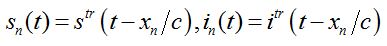 (79)
(79) (80)
(80)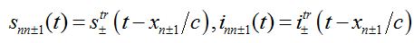 (81)
(81)where c is the epidemic speed, xn=n?x are the epidemic centra locations, ?x is the distance between centra (assume them to be equal for simplicity). Here itr(t), str(t) are the shares of hosts in node
 are the shares of guests in node n=0 arrived from node
  are the shares of guests in node n=0 arrived from node n = +1,
  are the shares of guests in node n=1 arrived from node
  are the shares of guests in node n=1 arrived from node n=0 where T=?x/c is the time lag between outbreaks in two neighbor nodes.
Substituting (79)-(81) into (75)-(78) we obtain the system of ODEs
 (82)
(82) (83)
(83) (84)
(84)A travelling wave should satisfy the initial conditions (dynamic equilibrium in the absence of outbreak):
 ,
,  ,
,  ,
, 
Here
 is the share of guest susceptibles at equilibrium in the absence of an outbreak. Normally it equals , i.e. the share of guest susceptibles at equilibrium in the absence of an outbreak [16]. We analyze of the influence of guest susceptibles before the outbreak by equating to to ε or to 0.When t → - ∞ travelling wave initially has exponential growth. We substitute the solution in the form
into (82)-(85) and linearize the equations with respect to
 .The values i, i-, i+ satisfy the following system of linear algebraic equations
 (87)
(87) (88)
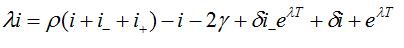
(88)Which has the following characteristic equation
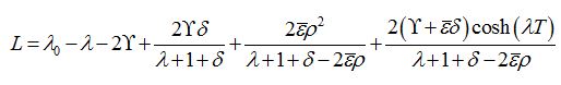
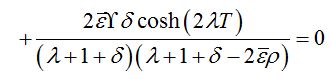
where λ0=ρ-1 is the initial growth rate of the limiting solution in the dimensionless time t′ = αt. In the case
=0 we have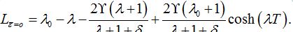 (89)
(89)By analogy with [13] (Eq. (42) there) we express these formulas in terms of γ and δ
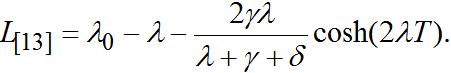 (90)
(90)The latter two formulas have some similarities but do not coincide exactly.
In accordance with the principle of Linear Spreading Velocity (LSV) [21-24] and also [13] we solve the system L = 0, ∂L / ∂λ with respect to λ and T.
The results from numerical exercises are shown in figure 4 with λ0T vs λ0τ for different ? = γ / (γ+δ) and ρ (solid color lines) where λ0 =ρ-1 is the initial growth rate for an individual SIR node in the SIC approximation. Recall that in terms of dimensional parameters they are (ρ-1) α T and
 respectively. Here dashed color curves are plotted for the case = 0, i.e., neglecting guest susceptibles before the outbreak. Also curves obtained in from eq. (90) are plotted by black lines. We make the following observations:
- Note that the functions λ0T (λ0τ ) depend on ρ but not to a large extent: the smaller the coupling ? - the smaller dependence. More discrepancy is observed for small τ.
- The curves for = 0 are very close to those obtained in [13], especially for small ?.
- Taking account of pre-outbreak guest susceptibles ( ≠ 0) noticeably shortens the time lag, i.e., it accelerates the propagation of the epidemic.
CONCLUSION
The mathematical modeling of epidemic processes using ODEs has a long history [1-3,24]. There is a plethora of models accounting for different aspects of the process, and it may be surprising that some aspects are still overlooked. To the best of our knowledge, the effect described here, on the speed of epidemic spread found in a model that introduces a proper account for the different migrations of hosts and guests is just another confirmation that the basic models are rich enough to reveal interesting new features. It is fair to argue that the advantages of considering host and guest separately has not been fully exploited, with many possibilities for the incorporation of heterogeneities within the population. For example, the infection and recovering rates βn; βmn; αn; αmn may be different for host and guest species. If, for hosts they are αmn and βmn for guests, this can be straightforwardly accounted in the proposed model by generalizing eqs. (7)-(10).

Analysis of this more general model, and further additions, will be given in subsequent works, but here we argue that a proper account of migration is the minimal amendment to make the model consistent. Another important aspect to recognize when model building is that precisely this model serves as a hydrodynamic limit of a natural Markov chain model presented in [15,16].
In this paper, we have explored analytically and numerically the SIR epidemic processes on a system of linked centra, and investigated the importance of population structure, specifically migration processes, on the developing dynamics of a directly transmitted infection. The analysis is performed in the framework of our previous SIC approximation, which impose a number of specific assumptions (discussed in section 8). With this reservation, the characteristics of epidemic speed and epidemic waveform pattern have been investigated in their most general aspects and the following conclusions have been drawn.
- An accurate account of the migration processes is crucial, even in a pure migration model without infection, to bring the qualitative behavior of the model consistent in line with an intuitive interpretation.
- The deterministic model of the migration process between two population centra demonstrates the different role of susceptibles and infectives in the epidemic spread across the population as a whole.
- The careful consideration of this simplified deterministic model allows us to derive the characteristic equation and hence to evaluate the speed of epidemic propagation via the chain of similar nodes. The appearance of pre-outbreak susceptibles accelerates the propagation of epidemic.
- The model demonstrates that the epidemic speed is dependent on reproduction number ρ but not to a large extent, and this dependence declines to zero when the coupling vanishes.
- The estimation of phenomenological parameters of the deterministic model ? and τ requires disease specific data. However, the study of pure migration (via questionnaire or transport data) can be related to parameters and γ and δ.
It is important to consider the behavior of such models in light of stochastic modeling that may often be considered the more realistic approach. First, we note that our model serves as a hydrodynamic approximation for a Markov process describing fluctuations of the discrete numbers of all types of individuals involved. In the framework of stochastic models γ and δ are treated as the transition rates, or probabilities of movements of a specific individual to a different center [16].
Second, we note that the epidemic can be described as a so-called branching process, in particular at the contamination stage. An accurate analysis of the basic reproduction number in the framework of a branching process model with discrete time in given in [25]: ρn is the mean number of infected susceptibles by initially infected individuals during his lifetime. It is proved that where Xk is the number of infected at the step k, It means that In this sense and (62) may be looked at as an expansion of ln ρ1 for adjusted for the time step ?t = 1/α1.
A focus for future work will be to estimate the influence of random fluctuations on epidemic speed and discuss the more complicated situation of a network with several routes of introduction of contamination in any particular population centre.
REFERENCES
- Kermack WO, McKendrick AG (1927) A contribution to the mathematical theory of epidemics. Proceedings of the Royal Society A: Mathematical, Physical and Engineering Sciences 115: 700-721.
- Murray JD (1993) Mathematical Biology. Springer, London, UK.
- Daley DJ, Gani JM (1999) Epidemic Modeling: An Introduction. Cambridge University Press, Cambridge, UK
- Burton J, Billings L, Cummings DA, Schwartz IB (2012) Disease persistence in epidemiological models: the interplay between vaccination and migration. Math Biosci 239: 91-96.
- Bolker B, Grenfell B (1995) Space, persistence and dynamics of measles epidemics. Philos Trans R Soc Lond B Biol Sci 348: 309-320.
- Grenfell BT, Bjørnstad ON, Kappey J (2001) Travelling waves and spatial hierarchies in measles epidemics. Nature 414: 716-723.
- Grenfell BT, Kleczkowski A, Gilligan CA, Bolker BM (1995) Spatial heterogeneity, nonlinear dynamics and chaos in infectious diseases. Stat Methods Med Res 4: 160-183.
- Riley S (2007) Large-scale spatial-transmission models of infectious disease. Science 316: 1298-1301.
- Colizza V, Vespignani A (2007) Invasion threshold in heterogeneous metapopulation networks. Phys Rev Lett 99: 148701.
- Colizza V, Vespignani A (2008) Epidemic modeling in metapopulation systems with heterogeneous coupling pattern: theory and simulations. J Theor Biol 251: 450-467.
- Arino J, Jordan J, van den Driessche P (2007) Quarantine in a multi-species epidemic model with spatial dynamics. Mathematical Biosciences 206: 46-60.
- Sazonov I, Kelbert M, Gravenor MB (2008) The speed of epidemic waves in a one-dimensional lattice of SIR models. Mathematical Modeling of Natural Phenomena 3: 28-47.
- Sazonov I, Kelbert M, Gravenor MB (2011) Travelling waves in a network of SIR epidemic nodes with an approximation of weak coupling. Math Med Biol 28: 165-183.
- Kelbert M, Sazonov I, Gravenor MB (2011) Critical reaction time during a disease outbreak. Ecological Complexity 8: 326-335.
- Sazonov I, Kelbert M, Gravenor MB (2011) A two-stage model for the SIR outbreak: accounting for the discrete and stochastic nature of the epidemic at the initial contamination stage. Math Biosci 234: 108-117.
- Sazonov I, Kelbert M (2015) Randomized migration processes between two epidemic centers. 1-27.
- Suhov Y, Kelbert M (2008) Probability and Statistics by Example: II Markov Chains: A Primer in Random Processes and their Applications. Cambridge University Press, Cambridge, UK.
- Wang W, Zhao XQ (2004) An epidemic model in a patchy environment. Math Biosci 190: 97-112.
- Wang W, Mulone G (2003) Threshold of disease transmission in a patch environment. J Math Anal Appl 285: 321-335.
- Arino J, Davis J, Hartley D, Jordan R, MillerJ, et al. (2005) A multi-species epidemic model with spatial dynamics, Math Med Biol-A Journal of the IMA 22: 129-142.
- Volpert AI, Volpert VA, Volpert VA (2000) Traveling Wave Solutions of Parabolic Systems (Volume 22), Mathematical Surveys and Monographs, American Mathematical Society, USA.
- van den Borsch F, Metz JAJ, Diekmann O (1990) The velocity of spatial population expansion. J Math Biol 28: 529-565.
- Mollison D (1991) Dependence of epidemic and population velocities on basic parameters. Math Biosci 107: 255-287.
- Mollison D (1995) Epidemic Models: Their Structure and Relation to Data, Cambridge University Press, Cambridge, UK.
- Pellis L, Ball F, Trapman P (2012) Reproduction numbers for epidemic models with households and other social structures. I. Definition and calculation of R0. Math Biosci 235: 85-97.
Citation: Sazonov I, Kelbert M, Gravenor MB (2015) A New View on Migration Processes between SIR Centra: An Account of the Different Dynamics of Host and Guest. J Infect Non Infect Dis 1: 003.
Copyright: © 2015 Igor Sazonov, et al. This is an open-access article distributed under the terms of the Creative Commons Attribution License, which permits unrestricted use, distribution, and reproduction in any medium, provided the original author and source are credited.