Effect of Treatment on Transmission Dynamics of SARS Epidemic
*Corresponding Author(s):
Afia NaheedMathematics Department, Ripha Institute Of Computing And Applied Sciences (RICAS), Riphah International University, Lahore, Pakistan
Tel:+92 03111747424,
Email:afia_naheed@yahoo.com
Abstract
Infectious diseases are the focus of much attention nowadays. Spatio-temporal study of the spread of their pathogenes is proving very helpful in developing strategies to control them, especially in cases where little biological information and treatment is available. The present work is based on the numerical study of Severe Acute Respiratory Syndrome (SARS) using an open population model consisting of six compartments. Different population distributions are used to generate the numerical simulations for the disease in different situations. Stability of the system is analysed. To see the effect on disease transmission different possible cases are studied in the absence and presence of diffusion in the system. Impact of treatment on the transmission of disease is analysed.
Keywords
INTRODUCTION
Recent years have seen an increasing trend of utilizing mathematical models for the prediction of and insight in infectious diseases. These models are considered as conceptual tools to explain the behavior of disease at different scales, and allow us to understand the spread of infection in the real world and the impact of various factors on disease dynamics. The key concepts associated with mathematical modeling, such as basic and effective reproduction number, generation time, epidemic growth rates, mortality rates, transmission rates, incubation periods, heterogeneities, disease transmission routes, risk factors for diseases spread and pre-clinical infectiousness play significant roles in the epidemiological analysis and control of diseases. The process of modeling in epidemiology has, at its heart, the same underlying philosophy and goals as ecological modeling. Both endeavors share the ultimate aim of attempting to understand the prevalence and distribution of a species, together with the factors that determine incidence, spread, and persistence [1,2].
The spatio-temporal spread of infectious diseases is the most significant area of epidemic modeling. Accurate and precise mathematical models enable scientists to understand the risk factors of disease transmission and to develop workable control strategies for possible future outbreaks. There are obvious public health and/or economic benefits in understanding the infectious dynamics of diseases in humans, animals and plants. Furthermore, it is well understood how important the spatial aspect of these dynamics is to understand disease spread [3]. In the case of emerging and re-emerging outbreaks of an infectious disease, it is crucial to quantify the characteristics of a disease in order to estimate the potential threat. Accurate estimation of these characteristics relies on modified epidemiological information.
Severe Acute Respiratory Syndrome (SARS) is one of the first pandemics of the 21st century. The World Health Organization (WHO) issued a global alert for SARS on 12th March 2003, at which point there were 150 suspected cases in 7 countries. The epidemic emerged in Guangdong Province in mainland China in November 16, 2002 and, on February 26 of the following year, new reports of SARS outbreaks came from Hong Kong and Vietnam. This contagious disease spread across the world through air travel and, as of June 13, 2003, the cumulative number of probable cases of SARS worldwide, reached 8,454 with 792 deaths [4]. Hong Kong bore a large proportion of this mortality and morbidity burden. In Hong Kong alone, 1755 probable SARS cases and 302 SARS related deaths were recorded from 15 February to 31st May 2003. SARS was caused by a coronavirus called SARS-Cov. As SARS was not previously endemic in humans, it seemed likely that SARS-Cov was a virus of animals that had crossed the species barrier to humans in the recent past [5]. Having originated in animals the virus then became efficient at human-to-human transmission which helped to develop the disease around the globe. SARS was brought under control at the end of 2003 but in 2004 a few cases emerged, either by accidental release of the virus from laboratories or from infected animals. It is difficult to make predictions regarding the resurgence of SARS, but current information suggests that the greatest risk of the reemergence of the disease may derive from animal reservoirs [5]. Recently, in 2012, a group of international scientists has found a SARS-like virus retrieved from a Chinese horseshoe bat, giving weight to the theory that these bats are the ultimate source of the virus that killed more than 900 people around the globe in 2003 [6].
Although much effort has been devoted to find the cure for SARS, there are still no effective drugs or vaccines for the disease. In this situation mathematical modeling permits the quantitative assessment of the epidemic potential of SARS and the effectiveness of measures, used to control disease transmission. Donnelly et al. [7] assessed the epidemiology of SARS in Hong Kong. They estimated the key epidemiological parametric distributions using integrated data bases constructed from several sources. These data bases contain information about epidemiological, demographic and clinical variables and provided the baseline for the parameters of SARS models by Chowell et al., [8,9], Gummel et al., [10], Riley et al., [11], Yan et al., [12] and Lipstich et al. [13]. Chowell et al., [8] fitted a compartmental model for the SARS epidemic to the data from Toronto, Hong Kong and Singapore. Chowell predicted the behavior of the disease and the role of diagnosis and isolation as a control mechanism in these regions, showing the differences among the epidemic dynamics occurred in these three cities. Riley et al., [11] and Lipstich et al., [13] used dynamic models for the respective transmission dynamics of SARS in Hong Kong and Singapore. Even though these models were complex, they allowed researchers to calculate numerous epidemiologically important parameters in order to assess the potential danger of the epidemic. Wallinga and Teunis [14] developed a likelihood-based estimation procedure that infers the temporal pattern of effective reproduction numbers from an observed epidemic curve. Zhou Y et al., [4] formulated a discrete mathematical model to investigate the transmission of SARS and estimated the parameters of the model on the basis of statistical data. Numerical simulations describing the transmission process for SARS in China have been carried out. Wang W and Ruan S proposed a mathematical model to simulate the SARS outbreak in Beijing by estimating the reproduction number and other important epidemiological parameters using the available data [15]. Xia et al., analysed the pattern of SARS and predicted the course of the SARS epidemic by establishing a compartmental model using data from Guangdong and Hong Kong [16]. Yang et al., also used a compartmental model to describe the SARS epidemic in spatio-temporal dimensions to determine whether people travelling in buses and trains infect one another or not [17]. They concluded that SARS can spread through people travelling in buses and trains.
Any treatment of infectious disease, SARS can give rise to many important questions such as, how treatment will effect disease transmission dynamics? Will it help to control the disease? Will the intensity of the disease be same or not. In order to answer such questions, we have developed an SEIJTR model for SARS in this paper. Here we investigate the transmission of SARS in the presence of treatment. A treatment class is included in the previous SEIJR model [18]. The values of the new parameters are calculated for the SARS epidemic using the data that appeared in Hong Kong 2003 [19]. This compartmental model includes susceptible, exposed, infected, diagnosed, treated and recovered classes. Diffusion has been included in the system to examine its role in transmission of the disease. The compartmental model for SARS transmission is given in section 2. The numerical scheme to solve the model is described in section 3. The stability of numerical model with and without diffusion is analysed in section 4. section 5 shows numerical simulations. Further discussions and conclusions are given in section 6.
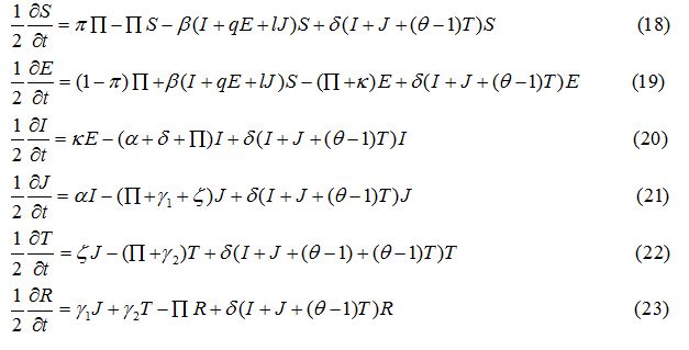
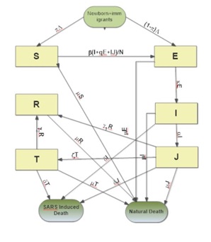
SEIJTR EPIDEMIC MODEL
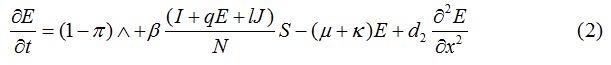
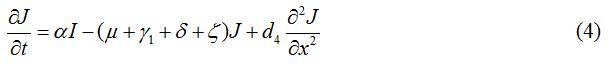
Equations


| Parameter | Description | Value | Source |
| Λ | Rate at which new recruits enter the population | 0.00002 per day | [19] |
| π | Proportion of new recruits into the population that are susceptible (the complementary proportion are infective) | 0.85 | [19] |
| β | Transmission coefficient | 0.24 | [19] |
| µ | Rate of natural mortality | 0.000035 | [10] |
| l | Relative measure of reduced risk among diagnosed | 0.65 | [19] |
| κ | Rate of progression from exposed to the infective | 0.195 | [19] |
| q | Relative measure of infectiousness for exposed individuals | 0.1 | [7] |
| α | Rate of progression from infective to diagnosed | 0.238 | [19] |
| γ1 | Natural recovery rate | 0.046 | [19] |
| γ2 | Recovery due to treatment | 0.05 | [19] |
| ζ | Treatment rate | 0.2 | [19] |
| δ | SARS-induced mortality rate | 0.024 | [19] |
| θ | Effectiveness of drugs as a reduction factor in disease-induced death of infectious individuals(0 ≤ θ ≤ 1) | 0.25 |  [19] |
Table 1: Biological definition and values of parameters.
Initial and boundary conditions


((S0, E0, I0, J0, T0, R0)| S0=0.97 Sech (-5x-1)2), E0 = J0 = T0 = R0 = 0, I0 = 0.03 exp (-5(x+1) 2), -2 ≤x ≤ 2) (16)
((S0, E0, I0, J0, T0, R0)| S0=0.96 Sech (15x), E0 = J0 = T0 = R0 = 0, -2 ≤ x ≤ 2
I0 = 0, -2 ≤ x < -0.6 and -0.6 < x < 2, I0 = 0.04, -0.6 ≤ x ≤ 0.6 (17)
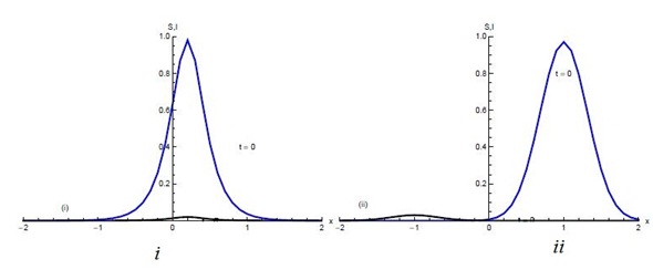
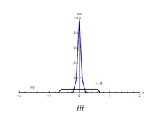
Figures 1 and 2 show the initial “population distributions" for S and I. A larger susceptible and a smaller infected proportion is concentrated towards the right half of the main domain in initial condition (i). In initial condition (ii), I has high concentration in the left half of the domain [-2,2] and population S has concentration on the right half of the domain [-2,2]. In the initial condition (iii) susceptible S exists in high concentration around the middle of domain [-2,2] with infected also around the middle but beyond the domain of S.
NUMERICAL SCHEME
Operator splitting method has been used to solve the SEIJTR model. According to this technique the system of equations is divided into nonlinear reaction equations and linear diffusion equations [20]. The nonlinear reaction equations to be used for the first half-time step are given as:
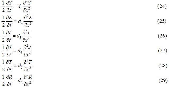
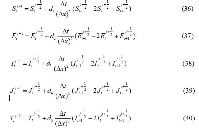
The second group consists of the linear diffusion equations, to be used for the second half-time step as follows:
Applying the forward Euler scheme the non-linear equations transform to
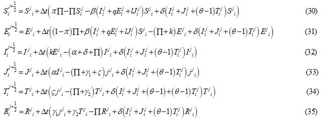
forward Euler scheme the non-linear equations transWhere 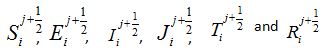 and are the approximated values of S, E, I, J, T and R at position -2+i∆x, for i = 0,1….. and time j∆t, j = 0,1,……. and
 and denote their values at the first half-time step. Similarly, for the second half-time step, the linear equations transform as
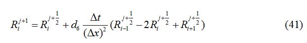
The stability condition satisfied by the numerical method described above is given as:
In each case, ∆x = 0.1, d1 = 0.025, d2 = 0.01, d3 = 0.001, d4 = 0.0, d5 = 0.0, d6 = 0.0 and ∆t = 0.03 are used.
STABILITY ANALYSIS
Disease-Free Equilibrium (DFE)
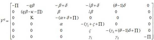
Trace [V0] = -α = + qβ – γ1 – γ2 – δ – ζ + δ(θ – 1) – κ - 6П < 0,
Det [V0] = B × П2 × A, where B = δ(θ – 1) - γ2 – П
and A = qβ (α+ δ + П) (γ1 – ζ – П) + βκ (lα + γ1 + ζ + П) – (κ + П) (α + δ + П) (γ1 + ζ + П)
As 0 < θ < 1 θ – 1 < 0 δ(θ – 1) < 0 δ(θ – 1) - γ2 – П) < 0, B < 0,
and for R0 < 1, A < 0, Hence, Det [V0] > 0.
Where
This shows that P0 is stable for R0 < 1. In the same way we can illustrate the stability of the endemic point for R0 > 1.
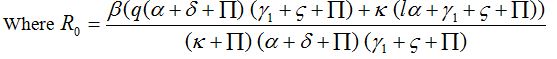
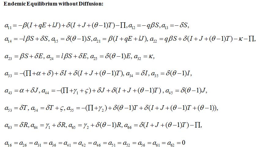
ENDEMIC EQUILIBRIUM WITHOUT DIFFUSION
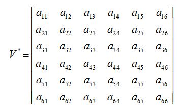
a11, a12,...a66 are given in appendix B
The characteristic equation for P* (S*, E*, I*, J*, T*, R*) can be written as

where p1, p2, p3, p4, p5, p6 and the Routh-Hurwitz conditions are calculated on the basis of [21] and are given as:
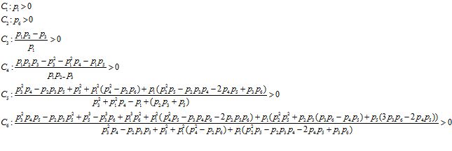
Here, p1, p2, p3, p4, p5 and p6 are the points of equilibrium given as:
P1 = (0.449403, 0.000058, 0.000043, 0.000042, 0.000122, 0.386452)
P2 = (0.546041, 0.000048, 0.000035, 0.000034, 0.000100, 0.318624)
P3 = (0.402087, 0.000064, 0.000061, 0.000044, 0.000131, 0.419654)
P4 = (0.373092, 0.000066, 0.000049, 0.000047, 0.000139, 0.440013)
P5 = (0.483878, 0.000054, 0.000033, 0.000039, 0.00012, 0.362260)
The numerical values of C1, C2, C3, C4, C5 and C6 on these points of equilibrium are given in table 5 in appendix A.
| Case | Equilibrium Point | C1 | C2 | C3 | C4 | C5 | Â C6 | Stable/Unstable |
| 1 |  P1 | 0.76036 |  4.27×10 -13 | 0.16736 | 0.01172 | 0.00024 | 2.54×10 -8 | Stable |
| 2 | P2 | 0.76123 | 3.26 ×10 -13 | 0.12823 | 0.01237 | 0.00029 | 2.16×10⁻⁸ | Stable |
| 3 | P3 | 0.70199 | 3.79 ×10⁻¹³ | 0.10024 | 0.00937 | 0.00017 | 2.19×10⁻⁸ | Stable |
| 4 | P4 | 0.75987 | 5.57 ×10 -13 | 0.126709 | 0.01133 | 0.00021 | 3.10×10⁻⁸ | Stable |
| 5 | P5 | 0.81903 | 4.77×10 -13 | 0.15788 | 0.01417 | 0.00031 | 2.93×10⁻⁸ | Stable |
Table 5: Routh-Hurwitz criteria of equilibrium without diffusion.
Endemic equilibrium with diffusion
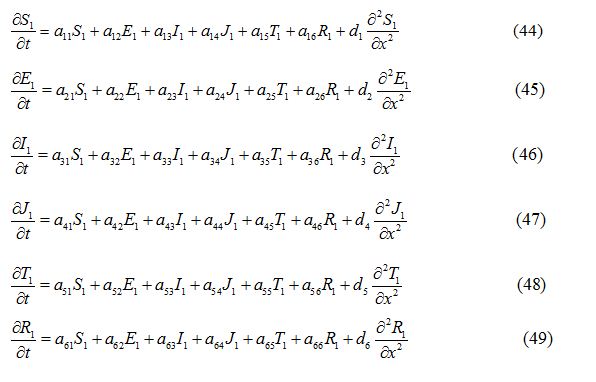
where a11, a12, a13…etc are the elements of the variational matrix V* calculated using the method described in [24]. We assume the existence of a Fourier series solution of equations (44) - (49), of form:
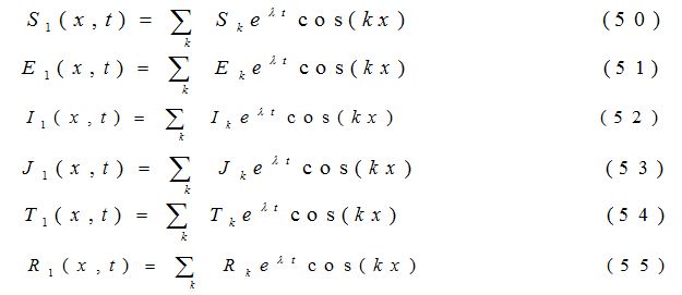
where k = , (n = 1, 2, 3,……) is the wave number for node n. Substituting the values of S1, E1, I1, J1, T1 and R1 into the equations (44) -(49), the equations are transformed into
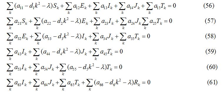
The variational matrix V for the equations (56) - (61)
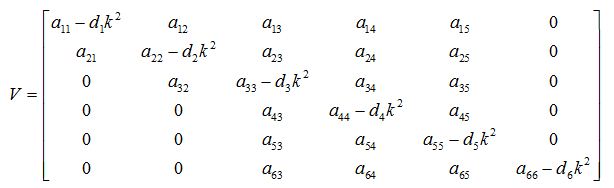
The characteristic equation for the variational matrix V is given as

where q1, q2, q3, q4 and q5 and q6 are calculated by the technique used in [24]. The Routh-Hurwitz Conditions are given in appendix B. The numerical values of Routh-Hurwitz criteria on points of equilibrium in the presence of diffusion are given in table 6 in appendix A.
| Case | Equilibrium Point | C1 | C2 | C3 | C4 | C5 | C6 | Stable/ Un-stable |
| 1 | P1 | 0.84918 | 4.51×10- 10 | 0.21558 | 0.02271 | 0.00107 | 2.17×10⁻⁵ | Stable |
| 2 | P2 | 0.85005 | 5.15 ×10 -10 | 0.21667 | 0.02335 | 0.00115 | 2.48×10⁻⁵ | Stable |
| 3 | P3 | 0.79082 | 3.25 ×10⁻¹⁰ | 0.18731 | 0.01873 | 0.00084 | 1.59×10⁻⁵ | Stable |
| 4 | P4 | 0.84869 | 4.15×10⁻¹⁰ | 0.21495 | 0.02234 | 0.00103 | 1.99×10⁻⁵ | Stable |
| 5 | P5 | 0.90786 | 5.85×10⁻¹⁰ | 0.24482 | 0.02688 | 0.00131 | 2.79×10⁻⁵ | Stable |
Table 6: Routh-Hurwitz criteria of equilibrium with diffusion.
Excited mode and bifurcation value
f(β) = A + B + (CD + E) (63)
where A = q32q4q5 - q2q3q52 + q53 - q33q6 + q13q62, B = q12(q42q5 - q3q4q6 - 2q2q5p6), C = q1 (q22q52 + q2q3), D = - q4q5 + q3q6, E = q1q5 (-2q4q5 + 3q3q6). n = 1 represents the first mode of excitation as being closest to the β-axis. It is observed that the bifurcation value of transmission coefficient, β and rate of progression from infective to diagnosed, α increases with diffusion as compared to the system without diffusion.
NUMERICAL SOLUTIONS
| Case | Values Considered | Â | Bifurcation Values | |||
| Without Diffusion | With Diffusion | |||||
|  β |  α |  β |  α |  β |  α | |
| 1 | 0.242 | 0.238 | 0.330 | 0.071 | 0.376 | 0.088 |
| 2 | 0.182 | 0.238 | 0.272 | 0.050 | 0.309 | 0.087 |
| 3 | 0.242 | 0.179 | 0.320 | 0.051 | 0.365 | 0.083 |
| 4 | 0.303 | 0.238 | 0.399 | 0.062 | 0.453 | 0.110 |
| 5 | 0.242 | 0.298 | 0.341 | 0.087 | 0.387 | 0.115 |
Table 7: Bifurcation Values of α and β.
Solutions of SEIJTR model in the absence of diffusion (Case 1)
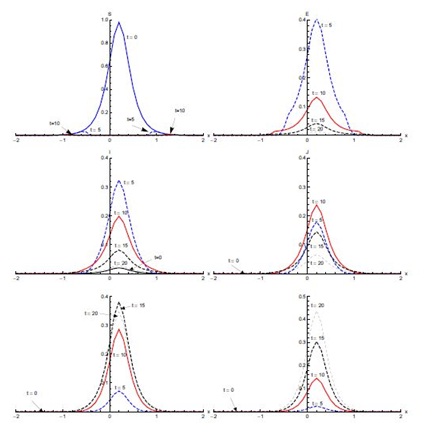
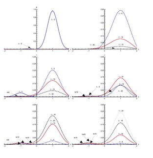
Figure 4, shows the output for initial condition (ii) in the absence of diffusion. The susceptible population, which is mainly concentrated in the domain [0,2], shows sharp decline in the first five days of the spread of SARS. After five days, concentration of susceptible is confined to the edges of the domain [0,2]. A small decrease is observed from t = 5 days onward (not visible in Figure 4). The exposed population grows in proportion remarkably fast in the first five days, showing that the rate of infection is very high during this period. Almost half of the susceptible population gets exposed to the disease in the first five days. Then the proportion of the population that is exposed rapidly decreases in the next five days. After t = 10 days, a slower decrease in exposed population proportion occurs. Most of the population becomes infective in the first five days and the domain of concentration of infective moves from [-2,0] to [0,2]. After t = 5 days, the infective proportion starts decreasing slowly till t = 10 days in the domain [0,2]. A sharp decline in infective proportion is observed in the whole domain [-2,2] between t = 10 days and t = 15 days, which continues at slow pace thereafter. The diagnosed proportion increases over the first five days. Between t = 5 and t = 10 days, an increase in diagnosed population proportion is noticed in the domain [0, 2]. In the same period, a much smaller proportion of diagnosed is also observed in the domain [-2,0]. A small proportion of the population is in the treatment class after five days and this proportion increases quickly in the next five days. The proportion of the population in treatment class reaches its maximum in t = 15 days and after that it decreases. There is negligible recovery in the first five days followed by a quicker recovery in the next five days in domain [-1.5,2], particularly the right half of the domain [-2,2]. The recovery proportion is greatest at t = 20 days.
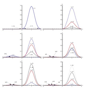
Figure 5 shows the results with initial condition (iii) in the absence of diffusion. In the first five days of the spread of SARS, the susceptible proportion reduces quickly to very low concentration around the edges at x = -0.1 and x = 0.1. In the first five days, most of the susceptible population gets exposed to the disease. After that, there is a quick decrease in the exposed population proportion until t = 10 days. This decreasing trend continues until t = 20 days in the domain [-0.1,0.1]. The infected population proportion increases quickly at a slower pace in the domain [-0.1,0.1] from its initial concentration in domain [-0.5,0.5] and reaches its peak value at t = 5 days. After that, infection decreases until t = 20 days. The diagnosed population proportion increases considerably in the first five days and is concentrated in the domain [-0.5,0.5]. The maximum diagnosed proportion occurs ten days after the onset of SARS. After t = 10 days, the diagnosed proportion of the population decreases. In the beginning, diagnosed individuals move slowly to the treatment class but a considerable increase in the proportion of the treated population is observed between t = 5 and t = 10 days. Recovery is extremely slow in first five days but during the next five days a substantial increase in the recovered population is observed, which continues till t = 20 days.
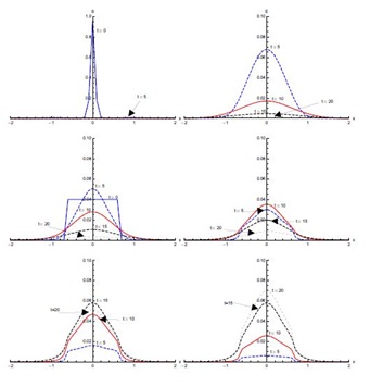
Solutions of SEIJTR model in the presence of diffusion (Case 1)
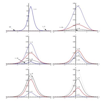
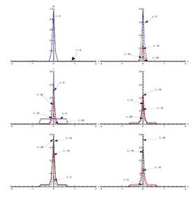
Figure 7, shows the solution for initial condition (ii) and with diffusion. Susceptible move from the domain [0,2] to the domain [-1.5,0] at t = 5 days and then to the domain [-2,-0.5] at t = 10 days (not clearly visible in Figure 7). The exposed population spread in the domain [-0.5,2]; attaining its maximum proportion at t = 5 days and then declining sharply in the next five days, spreading in the domain [-1,2]. After that there is slow decrease during the next ten days. Concentration of infected population remains mostly confined to the domain [-0.5,2] with a peak value at t = 5 days. After that, the infection proportion reduces gradually. At t = 20 days a very small proportion of the population is infected. The diagnosed population proportion also spreads in the domain [-0.5,2] with its maximum occurring at t = 10 days. A sharp increase in the treated population is observed from t = 5 days to t = 10 days in the domain [-2,2], mostly in the domain [-0.5,2]. The treated proportion of the population attains its peak value fifteen days after the spread of the disease and then reduces slowly. After fifteen days recovery seems to propagate in the larger domain [-2,2] but mostly in the domain [-0.5,2]. As compared to without diffusion case for recovered population, peak values are smaller but domain of concentration spreads.Figure 8, shows the solution for initial condition (iii) with diffusion. There is a quick decline in the susceptible population proportion during the initial five days of onset of disease. Maximum population exposure to SARS occurs in the domain [-1,1] in the first five days. Between t = 5 and t = 10 days, the peak value of the exposed population proportion decreases while the exposed spread in the domain [-1.5,1.5]. Infection peaks at t = 5 days and spreads in the domain [-1.5,1.5] at t = 10 days. Diffusion also causes diagnosed, treated and recovered population proportions to spread in the domain [-1.5,1.5] with peak values at t = 10, 15 and 20 days respectively.
Other cases
| Case | t | S(i) | S(ii) | S(iii) | E(i) | E(ii) | E(iii) | I(i) | I(ii) | I(iii) | R(i) | R(ii) | R(iii) |
| 1 | 00 | 0.980 | 0.970 | 0.960 | 0.000 | 0.000 | 0.000 | 0.020 | 0.030 | 0.040 | 0.000 | 0.000 | 0.000 |
| 05 | 0.034 | 0.039 | 0.009 | 0.406 | 0.455 | 0.393 | 0.324 | 0.313 | 0.322 | 0.024 | 0.014 | 0.026 | |
| 10 | 0.009 | 0.007 | 0.004 | 0.133 | 0.149 | 0.128 | 0.199 | 0.213 | 0.194 | 0.145 | 0.120 | 0.150 | |
| 15 | 0.004 | 0.003 | 0.002 | 0.041 | 0.047 | 0.040 | 0.082 | 0.090 | 0.079 | 0.305 | 0.275 | 0.309 | |
| 20 | 0.002 | 0.002 | 0.001 | 0.013 | 0.014 | 0.012 | 0.029 | 0.032 | 0.028 | 0.437 | 0.408 | 0.441 | |
| 2 | 00 | 0.980 | 0.970 | 0.96 | 0.000 | 0.000 | 0.000 | 0.020 | 0.030 | 0.040 | 0.000 | 0.000 | 0.000 |
| 05 | 0.053 | 0.070 | 0.009 | 0.423 | 0.479 | 0.409 | 0.324 | 0.309 | 0.322 | 0.021 | 0.012 | 0.024 | |
| 10 | 0.012 | 0.014 | 0.007 | 0.138 | 0.157 | 0.133 | 0.204 | 0.219 | 0.199 | 0.139 | 0.113 | 0.145 | |
| 15 | 0.005 | 0.006 | 0.002 | 0.043 | 0.049 | 0.042 | 0.085 | 0.094 | 0.082 | 0.299 | 0.267 | 0.305 | |
| 20 | 0.003 | 0.002 | 0.001 | 0.013 | 0.015 | 0.013 | 0.029 | 0.034 | 0.029 | 0.433 | 0.403 | 0.437 | |
| 3 | 00 | 0.980 | 0.970 | 0.960 | 0.000 | 0.000 | 0.000 | 0.020 | 0.030 | 0.040 | 0.000 | 0.000 | 0.000 |
| 05 | 0.034 | 0.039 | 0.009 | 0.407 | 0.373 | 0.394 | 0.456 | 0.352 | 0.372 | 0.019 | 0.011 | 0.022 | |
| 10 | 0.009 | 0.007 | 0.004 | 0.134 | 0.271 | 0.129 | 0.150 | 0.284 | 0.266 | 0.124 | 0.102 | 0.129 | |
| 15 | 0.004 | 0.003 | 0.004 | 0.042 | 0.131 | 0.041 | 0.048 | 0.141 | 0.127 | 0.276 | 0.247 | 0.281 | |
| 20 | 0.002 | 0.002 | 0.001 | 0.013 | 0.053 | 0.013 | 0.015 | 0.058 | 0.052 | 0.411 | 0.382 | 0.415 | |
| 4 | 00 | 0.980 | 0.970 | 0.960 | 0.000 | 0.000 | 0.000 | 0.020 | 0.030 | 0.040 | 0.000 | 0.000 | 0.000 |
| 05 | 0.008 | 0.037 | 0.008 | 0.217 | 0.439 | 0.383 | 0.191 | 0.315 | 0.322 | 0.025 | 0.016 | 0.028 | |
| 10 | 0.007 | 0.006 | 0.002 | 0.129 | 0.144 | 0.125 | 0.195 | 0.208 | 0.191 | 0.149 | 0.125 | 0.154 | |
| 15 | 0.003 | 0.002 | 0.001 | 0.040 | 0.045 | 0.039 | 0.079 | 0.087 | 0.077 | 0.308 | 0.279 | 0.313 | |
| 20 | 0.002 | 0.001 | 0.001 | 0.012 | 0.014 | 0.012 | 0.028 | 0.031 | 0.027 | 0.439 | 0.412 | 0.443 | |
| 5 | 00 | 0.980 | 0.970 | 0.960 | 0.000 | 0.000 | 0.000 | 0.020 | 0.030 | 0.040 | 0.000 | 0.000 | 0.000 |
| 05 | 0.035 | 0.039 | 0.009 | 0.406 | 0.456 | 0.393 | 0.284 | 0.279 | 0.281 | 0.028 | 0.016 | 0.031 | |
| 10 | 0.009 | 0.007 | 0.004 | 0.132 | 0.148 | 0.127 | 0.152 | 0.147 | 0.165 | 0.161 | 0.134 | 0.166 | |
| 15 | 0.004 | 0.003 | 0.002 | 0.041 | 0.046 | 0.039 | 0.056 | 0.054 | 0.061 | 0.323 | 0.293 | 0.328 | |
| 20 | 0.002 | 0.002 | 0.001 | 0.012 | 0.014 | 0.012 | 0.018 | 0.017 | 0.020 | 0.452 | 0.424 | 0.456 |
| Case | t | S(i) | S(ii) | S(iii) | E(i) | E(ii) | E(iii) | I(i) | I(ii) | I(iii) | R(i) | R(ii) | R(iii) |
| 1 | 00 | 0.980 | 0.970 | 0.960 | 0.000 | 0.000 | 0.000 | 0.020 | 0.030 | 0.040 | 0.000 | 0.000 | 0.000 |
| 05 | 0.00986 | 0.01191 | 0.00706 | 0.22313 | 0.29394 | 0.06802 | 0.18704 | 0.20155 | 0.05063 | 0.01379 | 0.00794 | 0.00613 | |
| 10 | 0.00108 | 0.00173 | 0.00129 | 0.05818 | 0.07859 | 0.01705 | 0.09902 | 0.12357 | 0.02796 | 0.08119 | 0.07235 | 0.02591 | |
| 15 | 0.00013 | 0.00067 | 0.00035 | 0.01584 | 0.02141 | 0.00467 | 0.03612 | 0.04704 | 0.01034 | 0.16517 | 0.16339 | 0.04998 | |
| 20 | 0.00008 | 0.00032 | 0.00017 | 0.00445 | 0.00593 | 0.00138 | 0.01168 | 0.01541 | 0.00343 | 0.23444 | 0.24169 | 0.07034 | |
| 2 | 00 | 0.980 | 0.970 | 0.960 | 0.000 | 0.000 | 0.000 | 0.020 | 0.030 | 0.040 | 0.000 | 0.000 | 0.000 |
| 05 | 0.01416 | 0.01892 | 0.01175 | 0.23344 | 0.31042 | 0.07408 | 0.18182 | 0.19248 | 0.04489 | 0.01161 | 0.0059 | 0.00552 | |
| 10 | 0.00171 | 0.00252 | 0.00201 | 0.06135 | 0.0835 | 0.01909 | 0.10112 | 0.12661 | 0.02878 | 0.07472 | 0.06503 | 0.02318 | |
| 15 | 0.00021 | 0.00096 | 0.00054 | 0.01679 | 0.02284 | 0.0053 | 0.03754 | 0.04916 | 0.01113 | 0.15645 | 0.15331 | 0.04589 | |
| 20 | 0.00009 | 0.00044 | 0.00023 | 0.00473 | 0.00635 | 0.00157 | 0.01226 | 0.01626 | 0.00378 | 0.22495 | 0.23083 | 0.06566 | |
| 3 | 00 | 0.980 | 0.970 | 0.960 | 0.000 | 0.000 | 0.000 | 0.020 | 0.030 | 0.040 | 0.000 | 0.000 | 0.000 |
| 05 | 0.00996 | 0.01204 | 0.00712 | 0.22348 | 0.29444 | 0.06814 | 0.21454 | 0.22479 | 0.05868 | 0.01100 | 0.00621 | 0.00499 | |
| 10 | 0.00109 | 0.00174 | 0.0013 | 0.05851 | 0.07904 | 0.01711 | 0.13599 | 0.16516 | 0.03819 | 0.06908 | 0.06095 | 0.02217 | |
| 15 | 0.00013 | 0.00068 | 0.00035 | 0.016 | 0.02165 | 0.00469 | 0.05891 | 0.07484 | 0.01665 | 0.14766 | 0.14526 | 0.04453 | |
| 20 | 0.00008 | 0.00032 | 0.00017 | 0.00451 | 0.00602 | 0.00138 | 0.02229 | 0.02882 | 0.00641 | 0.21674 | 0.22296 | 0.06451 | |
| 4 | 00 | 0.980 | 0.970 | 0.960 | 0.000 | 0.000 | 0.000 | 0.020 | 0.030 | 0.040 | 0.000 | 0.000 | 0.000 |
| 05 | 0.00759 | 0.00839 | 0.0049 | 0.21664 | 0.28347 | 0.06427 | 0.19018 | 0.20684 | 0.05379 | 0.01543 | 0.00955 | 0.00669 | |
| 10 | 0.00075 | 0.00132 | 0.00092 | 0.05618 | 0.07547 | 0.01587 | 0.09765 | 0.12152 | 0.02743 | 0.08576 | 0.07762 | 0.02799 | |
| 15 | 0.00009 | 0.00052 | 0.00025 | 0.01523 | 0.02049 | 0.00431 | 0.03522 | 0.04567 | 0.00987 | 0.17129 | 0.17053 | 0.05301 | |
| 20 | 0.00007 | 0.00025 | 0.00014 | 0.00427 | 0.00567 | 0.00127 | 0.01132 | 0.01487 | 0.00323 | 0.2411 | 0.24937 | 0.07383 | |
| 5 | 00 | 0.980 | 0.970 | 0.960 | 0.0000 | 0.000 | 0.000 | 0.020 | 0.030 | 0.040 | 0.000 | 0.000 | 0.000 |
| 05 | 0.00997 | 0.01206 | 0.00719 | 0.22333 | 0.29429 | 0.06821 | 0.16394 | 0.18103 | 0.043998 | 0.01612 | 0.00938 | 0.00704 | |
| 10 | 0.00109 | 0.00175 | 0.00131 | 0.05807 | 0.07846 | 0.01709 | 0.07468 | 0.09523 | 0.02127 | 0.09009 | 0.08086 | 0.02859 | |
| 15 | 0.00013 | 0.00068 | 0.00035 | 0.01576 | 0.02129 | 0.00468 | 0.02411 | 0.03193 | 0.00701 | 0.17671 | 0.17542 | 0.05352 | |
| 20 | 0.00008 | 0.00032 | 0.00017 | 0.00442 | 0.00589 | 0.00138 | 0.00712 | 0.00949 | 0.00213 | 0.24523 | 0.2531 | 0.07389 |
Discussion and Conclusion
| Case | β | α | Value of R0 |
| 1 | 0.242 | 0.238 | 1.6148 |
| 2 | 0.182 | 0.238 | 1.2212 |
| 3 | 0.242 | 0.179 | 1.8668 |
| 4 | 0.303 | 0.238 | 2.0354 |
| 5 | 0.242 | 0.298 | 1.4561 |
Table 4: Basic Reproduction Number R0
In initial condition (i), without diffusion, infectives are concentrated in the domain [-1,1]. With and without diffusion in the system, infection spreads quickly in the first five days of onset of disease. With diffusion in the system, infected population spreads to the edges of the domain [-2,2] in the first ten days, where initially there were no infectives. But a decrease in the peak values of the infected proportion occurs, showing that diffusion causes a decrease in the intensity of disease. Maximum population of diagnosed then enters treatment class at the day fifteen of the disease. In initial condition (ii), susceptible and infected proportions are in different domains initially. Here, infected not only increase with the passage of time but also move from domain [-2,0] to domain [0,2] without diffusion. With diffusion in the system, the infected spread to almost in the whole domain [-2,2]. Under initial condition (iii), there is a significant shift as the infected population move to the domain [-0.1,0.1] significantly from the initial domain [-0.6,0.6]. Diffusion again causes the infection to spread, in the domain [-1.5,1.5] but with reduced peak values.
• The spread of the disease is affected by variation in initial the population distribution.
• Transmission coefficient, β and rate of progression from infective to diagnosed, α play a crucial role in increasing or decreasing the basic reproductive number R0, thus affecting the degree of spread of disease.
• Diffusion reduces the peak values of the population in all compartments, thus reducing intensity of disease.
• Introduction of treatment immensely affects the transmission, making it faster and, in the process increasing recovery significantly [23].
ACKNOWLEDGMENT
One of the authors, Afia Naheed thanks Swinburne University of Technology for the Postgraduate Research Award.
REFERENCES
- Anderson RM, May RM (1979) Population biology of infectious diseases: Part I. Nature 280: 361-367.
- Earn DJ, Rohani P, Grenfell BT (1998) Persistence, chaos and synchrony in ecology and epidemiology. Proc Biol Sci 265: 7-10.
- Lawson AB (2001) Statistical Methods in Spatial Epidemiology. Int J Epidemiol 6: 1504-1505.
- Zhou Y, MA Z, Brauer F (2004) A Discrete Epidemic Model for SARS Transmission and Control in China. Math and Comput Model 40: 1491-1506.
- Peiris JS, Yuen KY, Osterhaus AD, Stöhr K (2003) The severe acute respiratory syndrome. N Engl J Med 349: 2431-2441.
- http://www.canada.com/health/SARSlike+viruses+found+Chinese+bats+closest+hits+2003+outbreak+virus/9102750/story.html
- Donnelly CA, Ghani AC, Leung GM, Hedley AJ, Fraser C, et al. (2003) Epidemiological determinants of spread of causal agent of severe acute respiratory syndrome in Hong Kong. Lancet 361: 1761-1766.
- Chowell G, Fenimore PW, Castillo-Garsow MA, Castillo-Chavez C (2003) SARS outbreaks in Ontario, Hong Kong and Singapore: the role of diagnosis and isolation as a control mechanism. J Theor Biol 224: 1-8.
- Chowell G, Castillo-Chavez C, Fenimore PW, Kribs-Zaleta CM, Arriola L, et al. (2004) Model parameters and outbreak control for SARS. Emerg Infect Dis 10: 1258-1263.
- Gumel AB, Ruan S, Day T, Watmough J, Brauer F, et al. (2004) Modelling strategies for controlling SARS outbreaks. Proc Biol Sci 271: 2223-2232.
- Riley S, Fraser C, Donnelly CA, Ghani AC, Abu-Raddad LJ, et al. (2003) Transmission dynamics of the etiological agent of SARS in Hong Kong: impact of public health interventions. Science 300: 1961-1966.
- Yan X, Zou Y, Li J (2007) Optimal quarantine and isolation strategies in epidemics control. World Journal of Modelling and Simulation 3: 202-211.
- Lipsitch M, Cohen T, Cooper B, Robins JM, Ma S, et al. (2003) Transmission dynamics and control of severe acute respiratory syndrome. Science 300: 1966-1970.
- Wallinga J, Teunis P (2004) Different epidemic curves for severe acute respiratory syndrome reveal similar impacts of control measures. Am J Epidemiol 160: 509-516.
- Wang W, Ruan S (2004) Simulating the SARS outbreak in Beijing with limited data. J Theor Biol 227: 369-379.
- Xia JL, Yao C, Zhang GK (2003) Analysis of piecewise compartmental modeling for epidemic of SARS in Guangdon. Chinese Journal of Health Statistics 20: 162-163.
- Yang H, Li XW, Shi H, Zhao KG, Han LJ (2003) Fly dots spreading model of SARS along transportation. J Remote Sens 7: 251-255.
- Naheed A, Singh M, Lucy D (2014) Numerical study of SARS epidemic model with the inclusion of diffusion in the system. Applied Mathematics and Computation. 229: 480-498.
- Naheed A, Singh M, Lucy D (2014) Parameter estimation with uncertainty and sensitivity analysis for the SARS outbreak in Hong Kong.
- Yanenko NN (1971) The Method of Fractional Steps: The Solution of Problems of Mathematical Physics in Several Variables. Springer Berlin Heidelberg, Germany.
- Meinsma G (1995) Elementary proof of the Routh-Hurwitz test. Systems & Control Letters 25: 237-242.
- Chakraborty A, Singh M, Lucy D, Ridland P (2007) Predator-prey model with prey-taxis and diffusion. Mathematical and Computer Modelling 46: 482-498.
- Sapoukhina N, Tyutyunov Y, Arditi R (2003) The role of prey taxis in biological control: a spatial theoretical model. Am Nat 162: 61-76.
- Samsuzzoha Md, Singh M, Lucy D (2010) Numerical study of an influenza epidemic model with diffusion. Applied Mathematics and Computation 217: 3461-3479.
APPENDIX B
Endemic Equilibrium without Diffusion:
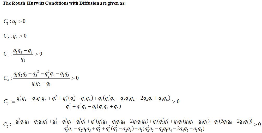
The Routh-Hurwitz Conditions with Diffusion are given as:
Citation: Naheed A, Singh M, Richards D (2016) Effect of Treatment on Transmission Dynamics of SARS Epidemic. J Infect Non Infect Dis 2:16.
Copyright: © 2016 Afia Naheed, et al. This is an open-access article distributed under the terms of the Creative Commons Attribution License, which permits unrestricted use, distribution, and reproduction in any medium, provided the original author and source are credited.