Comprehensive Assessment of Left Ventricular Wall Motion Abnormalities in Coronary Artery Disease Using Cardiac Magnetic Resonance
*Corresponding Author(s):
Ion CodreanuDepartment Of Physiology, University Of Oxford, Oxford, United Kingdom
Tel:+44 1865282246,
Fax:+44 1865282272
Email:codrion@yahoo.com.com
Ion Codreanu
Department Of Radiology, Medpark International Hospital, Nicolae Testemitanu State University Of Medicine And Pharmacy, Oxford, Republic Of Moldova
Tel:+44 1865282246,
Fax:+44 1865282272
Email:codrion@yahoo.com.com
Abstract
Objective: To obtain new details of three-dimensional Left Ventricular (LV) wall motion in patients with Coronary Artery Disease (CAD) using cardiac magnetic resonance navigator gated high temporal resolution tissue phase mapping.
Methods: LV motion patterns, myocardial velocities and time-to-peak values for radial, rotational and longitudinal motion were obtained in 19 patients with triple vessel CAD and in a group of 9 age-matched healthy subjects. Radial, circumferential and longitudinal velocity curves were recorded separately for 16 ventricular segments. Ventricular torsion rate and longitudinal strain rate were also derived for each group.
Results: Markedly reduced peak diastolic longitudinal velocities (-7.9 ± 0.6 versus -14.1 ± 1.1cm/s) and peak diastolic longitudinal strain rates (1.1 ± 0.2 versus 2.7 ± 0.1s-1) were the most prominent findings in CAD. Patients with CAD also demonstrated lower peak radial velocities, the difference increasing towards the LV apex (peak systolic values of 3.1 ± 0.2 versus 3.5 ± 0.2cm/s at the LV base and 2.4 ± 0.2 versus 3.5 ± 0.2cm/s at the LV apex), with sub-endocardial myocardium being affected to a greater extent. Prominent changes in rotational velocities and an altered pattern of ventricular rotation were also noted in CAD patients.
Conclusion: The study revealed complex alterations in radial, rotational and longitudinal LV wall motion in patients with CAD. Peak diastolic longitudinal velocity at the LV base and peak diastolic longitudinal strain rate seem particularly useful for detecting early changes in LV dysfunction associated to CAD. Evaluation of the pathophysiological interplays and underlying mechanisms of these changes require further studying and can provide new insights into understanding the pathophysiology of CAD.
Keywords
ABBREVIATIONS
CAD: Coronary Artery Disease
LV: Left Ventricular
MR: Magnetic Resonance
TPM: Tissue Phase Mapping
INTRODUCTION
Subtle changes in Left Ventricular (LV) wall motion patterns have diagnostic and prognostic value in patients with Coronary Artery Disease (CAD) [1-10], and can precede chest pain and electrocardiographic changes [11,12]. Additionally, ventricular strain rate measurements can improve assessment of myocardial viability [13]. For instance, combined assessment of subendocardial contractile impairment and post-systolic shortening (defined as the peak strain after end systole) was demonstrated to be useful in identifying hypoperfused myocardium in the absence of visual wall motion abnormalities [11]. Quantitative measurement of myocardium strain and myocardium strain rate showed promising results in the evaluation of infarct size in patients with anterior ST-Elevation Myocardial Infarction (STEMI) [14]. Segmental strain and strain rate measurements in longitudinal, radial and circumferential directions have also been reported useful for predicting the presence of coronary collateral circulation in the ischemic myocardium [15].
Cardiac Magnetic Resonance (CMR) provides a comprehensive evaluation for patients with CAD, including cardiac anatomy, function, viability and myocardial perfusion. Long and short axis cine images provide qualitative assessment of global and regional wall motion abnormalities, though the value of using CMR for comprehensive assessment of 3D regionality in CAD is not well established. Previously, we used the CMR navigator gated, high temporal resolution Tissue Phase Mapping (TPM) for investigating LV remodeling following Coronary Artery By-pass Graft surgery (CABG) [16]. Using the same methodology, subsequently, we investigated age related changes in regional and global myocardial wall motion in healthy individuals without cardiac disease [17]. In the current study, we aimed to compare three-dimensional LV wall motion in patients with CAD with similar data obtained in their age-matched healthy controls.
METHODS AND MATERIALS
Study population
The majority of patients had risk factors for CAD, including hypercholesterolaemia (15 patients), hypertension (12 patients), smoking (9 patients), diabetes mellitus (8 patients), and peripheral vascular disease (6 patients). All patients were receiving medical therapy, including lipid lowering medication (19 patients), ACE inhibitors (17 patients), aspirin (17 patients), beta blockers (15 patients) and diuretics (7 patients). In this group with CAD, Left Ventricular (LV) ejection fraction averaged 40.0 ± 2.5% (mean ± SD), cardiac output 5.6 ± 0.3 l/min, cardiac index 2.7 ± 1.2 l/min/m2, end systolic volume 151.5 ± 15.7 ml, end diastolic volume 244.2 ± 17.2 ml, LV mass 162.0 ± 13.9 g, LV mass index 80.1 ± 4.9 g/m2. Since CABG is expected to add a variety of confounding factors that affect LV wall motion, only the pre-CABG data were used in the current study.
A group of 9 age-matched healthy controls (66 ± 7 years old) were also studied. All healthy volunteers were non-smokers and underwent a medical assessment prior to acceptance in the study to exclude a history of cardiovascular and metabolic disease. Their baseline data have also been used in a separate study to investigate age-related changes in LV wall motion in healthy individuals [17]. The study was performed according to the principles of the declaration of Helsinki and was approved by a local clinical research ethics committee. Each subject provided written informed consent.
Cardiac MR scans
Tissue Phase Mapping (TPM) analysis was performed using customised software (MATLAB®, v. 6.5; MathWorks®, Natick, MA). The endocardial and epicardial borders were manually contoured for the base, mid ventricle and apex for each phase of the cardiac cycle. For the TPM analysis, the left ventricle was divided into 16 segments (6 basal, 6 middle and 4 apical) according to the American Heart Association model [24]. In-plane velocities were transformed into an internal polar coordinate system positioned at the centre of the mass of the left ventricle. Global ventricular velocity time courses for radial, circumferential and longitudinal motion were calculated for each group by averaging over the entire segmentation mask. In addition, graphical representations of all ventricular velocities during a cardiac cycle for individual LV segments were obtained. Global ventricular torsion and strain rates were also determined.
Statistical analysis
RESULTS
Radial motion
| LV level and myocardial layer | CAD patients | Healthy controls | p- value | CAD patients | Healthy controls | p-value | |
| Peak systolic radial velocity (cm/s) | Time to peak values (% of ES) | ||||||
| LV base | epicardial | 2.8 ± 0.2 | 3.1 ± 0.2 | 0.11 | 38.5 ± 2.0 | 42.7 ± 2.6 | 0.23 |
| transmural | 3.1 ± 0.2 | 3.5 ± 0.2 | 0.07 | 38.2 ± 2.1 | 42.6 ± 2.6 | 0.22 | |
| endocardial | 3.4 ± 0.2 | 4.0 ± 0.2 | 0.06 | 38.1 ± 1.9 | 43.6 ± 2.6 | 0.11 | |
| Mid-ventricle | epicardial | 2.7 ± 0.2 | 3.2 ± 0.3 | 0.11 | 36.8 ± 1.8 | 39.7 ± 1.4 | 0.33 |
| transmural | 3.0 ± 0.2 | 3.5 ± 0.3 | 0.06 | 39.6 ± 2.3 | 42.7 ± 2.1 | 0.42 | |
| endocardial | 3.3 ± 0.2 | 4.0 ± 0.3 | 0.04 | 41.1 ± 2.1 | 44.7 ± 1.5 | 0.28 | |
| LV apex | epicardial | 2.4 ± 0.2 | 3.2 ± 0.2 | < 0.01 | 38.8 ± 1.9 | 38.6 ± 1.9 | 0.97 |
| transmural | 2.4 ± 0.2 | 3.5 ± 0.2 | < 0.01 | 39.7 ± 1.9 | 39.1 ± 1.7 | 0.86 | |
| endocardial | 2.5 ± 0.2 | 3.8 ± 0.2 | < 0.01 | 44.3 ± 1.8 | 40.1 ± 1.4 | 0.17 | |
| Peak diastolic radial velocity (cm/s) | Time to peak values (% of ED) | ||||||
| LV base | epicardial | -3.4 ± 0.3 | -4.4 ± 0.4 | 0.03 | 18.9 ± 0.9 | 19.1 ± 1.8 | 0.90 |
| transmural | -3.8 ± 0.4 | -5.5 ± 0.4 | < 0.01 | 19.0 ± 0.9 | 18.8 ± 1.9 | 0.92 | |
| endocardial | -4.3 ± 0.4 | -6.6 ± 0.5 | < 0.01 | 19.1 ± 1.0 | 18.8 ± 1.7 | 0.85 | |
| Mid-ventricle | epicardial | -3.0 ± 0.3 | -4.3 ± 0.2 | < 0.01 | 23.8 ± 1.2 | 23.2 ± 1.2 | 0.78 |
| transmural | -3.3 ± 0.3 | -5.2 ± 0.2 | < 0.01 | 24.3 ± 1.4 | 23.5 ± 1.1 | 0.76 | |
| endocardial | -3.6 ± 0.3 | -6.1 ± 0.3 | < 0.01 | 24.1 ± 1.4 | 23.5 ± 1.1 | 0.80 | |
| LV apex | epicardial | -3.1 ± 0.3 | -4.2 ± 0.3 | 0.01 | 24.1 ± 1.3 | 27.4 ± 1.4 | 0.15 |
| transmural | -3.3 ± 0.3 | -4.7 ± 0.3 | < 0.01 | 24.3 ± 1.2 | 27.4 ± 1.4 | 0.16 | |
| endocardial | -3.5 ± 0.3 | -5.2 ± 0.4 | < 0.01 | 24.3 ± 1.2 | 27.4 ± 1.4 | 0.16 | |
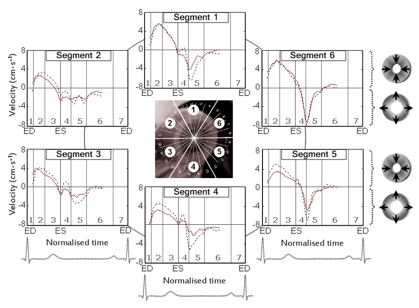
Figure 2: Radial velocity graphs for basal LV segments during a cardiac cycle.
Rotational motion
| LV level and myocardial layer | CAD patients | Healthy controls | p- value | CAD patients | Healthy controls | p-value | |
| Peak clockwise velocity (cm/s) | Time to peak values (% of ES) | ||||||
| LV base | epicardial | 2.4 ± 0.2 | 2.6 ± 0.3 | 0.35 | 51.2 ± 2.0 | 47.5 ± 1.1 | 0.25 |
| transmural | 2.3 ± 0.2 | 2.5 ± 0.3 | 0.27 | 51.5 ± 2.0 | 47.5 ± 1.1 | 0.21 | |
| endocardial | 2.2 ± 0.2 | 2.5 ± 0.3 | 0.24 | 51.2 ± 1.8 | 46.3 ± 1.1 | 0.10 | |
| Mid-ventricle | epicardial | 2.9 ± 0.4 | 2.0 ± 0.2 | 0.09 | 137.5 ± 2.3 |
101.2 ± 0.6† 147.5 ± 5.1† |
< 0.01 |
| transmural | 2.7 ± 0.4 | 2.0 ± 0.3 | 0.14 | 137.0 ± 2.2 |
99.7 ± 2.0† 147.5 ± 5.1† |
< 0.01 | |
| endocardial | 2.6 ± 0.4 | 2.2 ± 0.3 | 0.25 | 140.3 ± 3.2 |
99.7 ± 2.0† 147.5 ± 5.1† |
< 0.01 | |
| LV apex | epicardial | 4.0 ± 0.5 | 2.3 ± 0.3 | 0.02 | 137.1 ± 2.5 | 109.9 ± 4.6 | < 0.01 |
| transmural | 3.8 ± 0.5 | 2.2 ± 0.2 | 0.02 | 137.6 ± 2.5 | 109.9 ± 4.7 | < 0.01 | |
| endocardial | 3.6 ± 0.5 | 2.2 ± 0.2 | 0.03 | 135.3 ± 3.1 | 111.4 ± 5.1 | < 0.01 | |
| Peak counterclockwise velocity (cm/s) | Time to peak values (% of ED) | ||||||
| LV base | epicardial | -3.7 ± 0.4 | -3.3 ± 0.4 | 0.25 | 117.7 ± 2.1 | 117.6 ± 1.5 | 0.98 |
| transmural | -3.5 ± 0.4 | -3.3 ± 0.4 | 0.34 | 119.4 ± 1.9 | 118.1 ± 1.5 | 0.70 | |
| endocardial | -3.4 ± 0.4 | -3.4 ± 0.3 | 0.48 | 119.0 ± 2.0 | 118.6 ± 1.7 | 0.98 | |
| Mid-ventricle | epicardial | -3.8 ± 0.4 | -3.5 ± 0.4 | 0.34 | 27.8 ± 1.6 | 25.3 ± 1.9 | 0.39 |
| transmural | -3.6 ± 0.4 | -3.5 ± 0.3 | 0.44 | 27.2 ± 1.6 | 25.3 ± 1.9 | 0.51 | |
| endocardial | -3.4 ± 0.4 | -3.5 ± 0.3 | 0.46 | 27.6 ± 1.4 | 25.3 ± 1.9 | 0.41 | |
| LV apex | epicardial | -4.7 ± 0.4 | -3.8 ± 0.4 | 0.07 | 29.5 ± 1.3 | 26.2 ± 1.1 | 0.13 |
| transmural | -4.5 ± 0.4 | -3.7 ± 0.4 | 0.13 | 24.3 ± 1.2 | 26.2 ± 1.1 | 0.11 | |
| endocardial | -4.2 ± 0.4 | -3.7 ± 0.4 | 0.20 | 29.6 ± 1.3 | 26.7 ± 1.4 | 0.24 | |
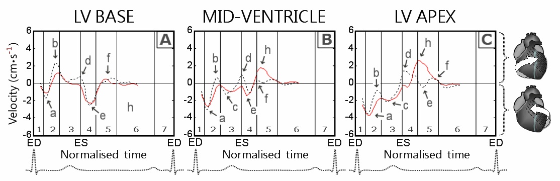
The time to peak counter-clockwise velocity at the LV apex and mid-ventricle in both control and CAD groups was represented by the initial counter-clockwise rotation of the entire ventricle (Figure 5 (B,C), arrow a), whilst at the LV base by the first wave of recoil counter-clockwise rotation of the LV base during untwisting (Figure 5A, arrow e).
Solid line - patients with CAD; Dotted line - healthy controls; Segments: 1 - basal anterior segment; 2 - basal anteroseptal segment; 3 - basal inferoseptal segment; 4 - basal inferior segment; 5 - basal inferolateral segment; and 6 - basal anterolateral segment; Cardiac cycle phases: 1 - isovolumetric contraction; 2 - rapid ejection; 3 - reduced ejection; 4 - isovolumetric relaxation; 5 - rapid filling; 6 - diastasis; and 7 - atrial systole; ED: End Diastole; ES: End Systole
The time to peak clockwise velocity at the LV base was represented in both groups by the clockwise rotation of the ventricular base during ejection (Figure 5A, arrow b). At the mid-ventricular level, the time to peak clockwise velocity in healthy controls was divided in accordance with two different waves of clockwise rotation located at 99.7% and 147.5% of end-systole (Figure 5B, arrows d and f, dotted line). In different subjects, the time to peak clockwise velocity at the mid-ventricle was represented by any of these two peaks, which is also reflected in table 2). In CAD patients, the time to peak clockwise velocity at the mid-ventricular level was represented by a single prominent wave of clockwise rotation transmitted from the apex (Figure 5B, arrow h, solid line). At the LV apex, the time to peak clockwise velocity in healthy controls was represented by the first recoil wave of clockwise rotation (Figure 5C, arrow d, dotted line), whilst in CAD patients-by the delayed wave of apical untwisting with a prominent single peak of clockwise recoil motion (Figure 5C, arrow h, solid line).
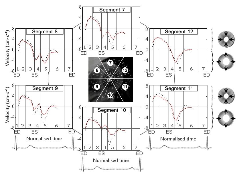
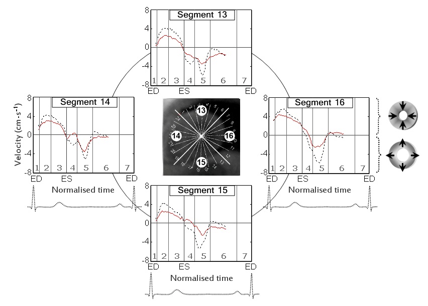
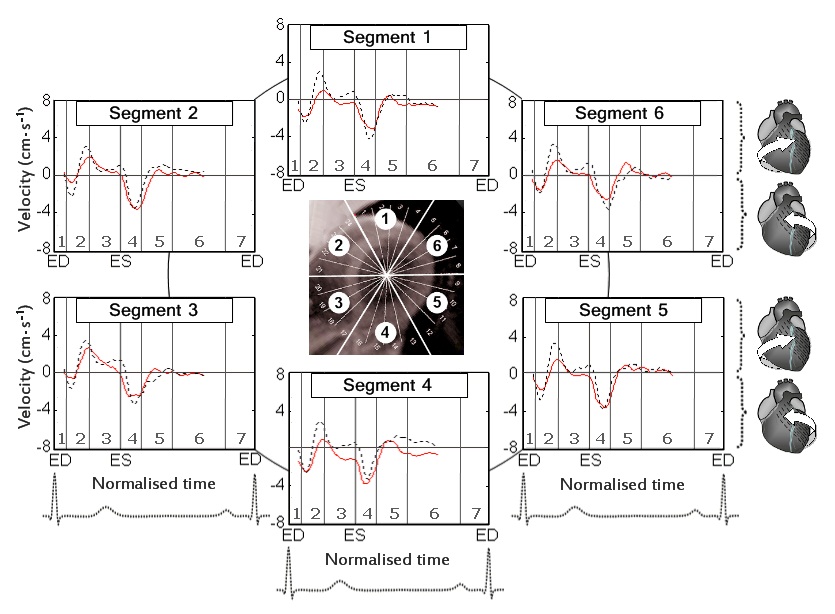
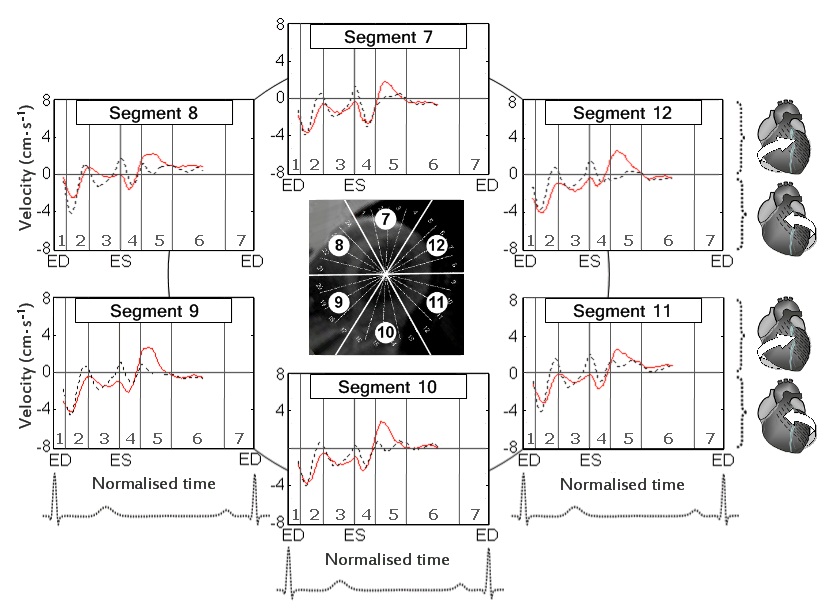
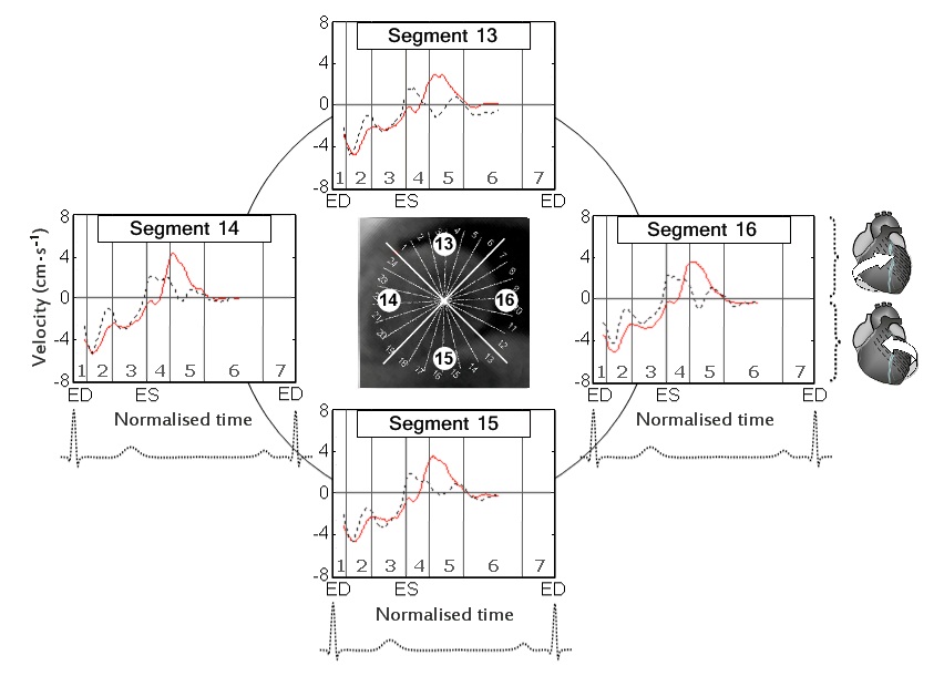
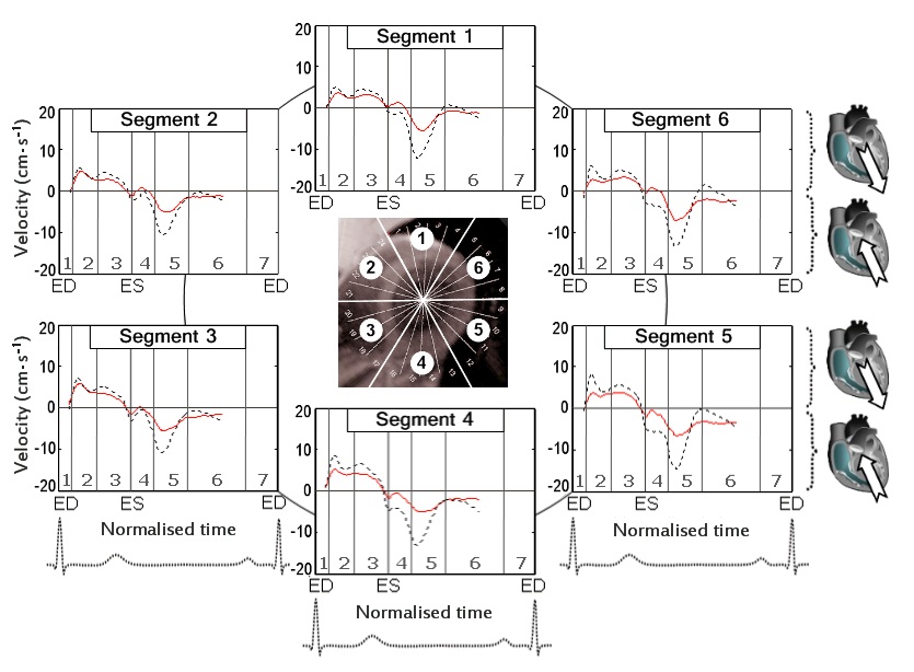
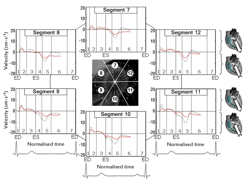
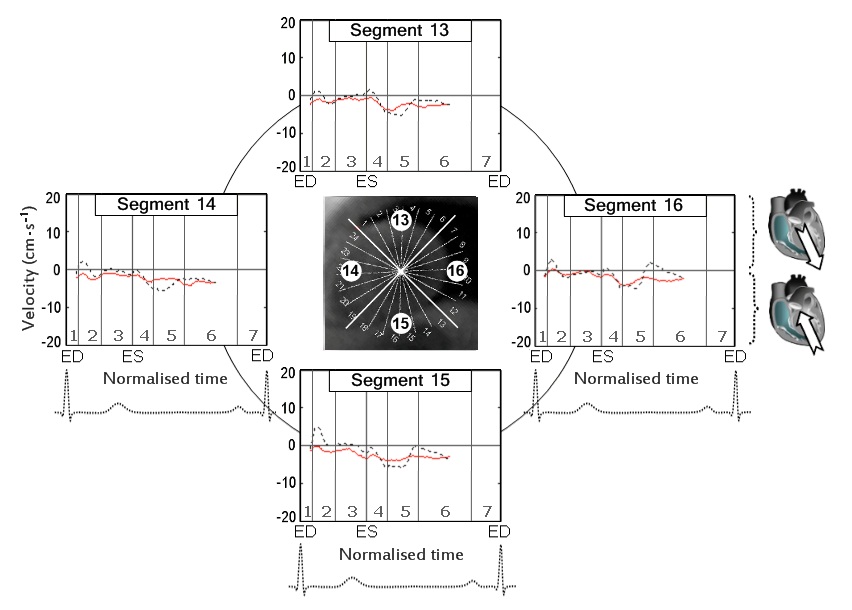
The circumferential velocities for individual ventricular segments at the LV base, mid-ventricle and LV apex are displayed in figure 6,7 and 8 respectively. An altered pattern of rotational motion is observed in patients with CAD, particularly affecting apical and, to a lower degree, mid-ventricular and basal LV segments.
Longitudinal motion
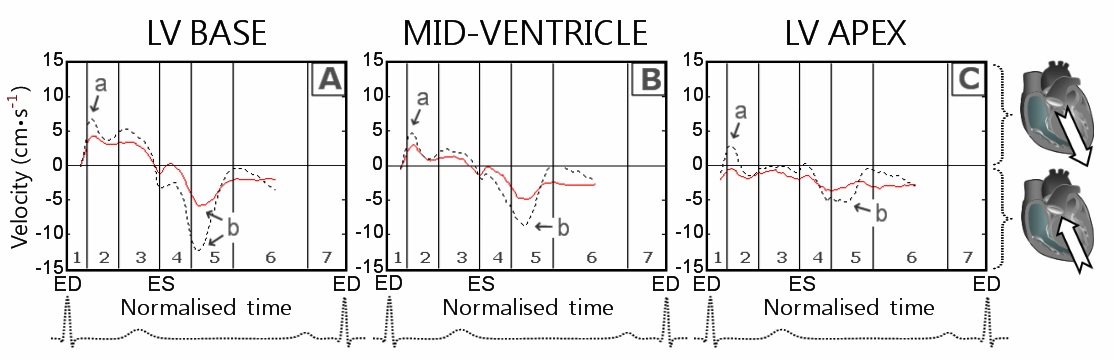
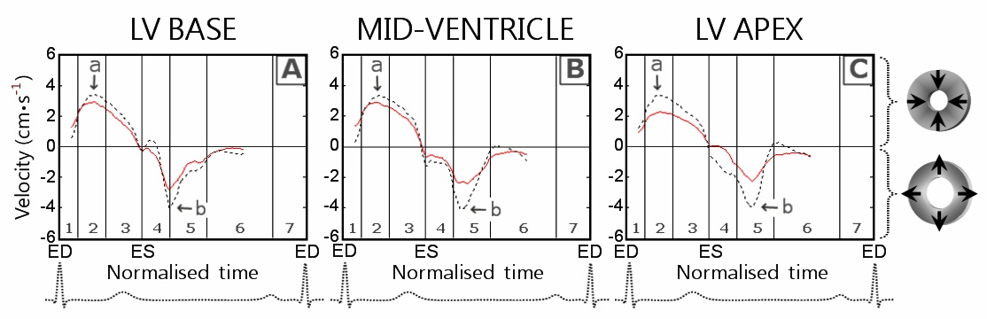
Figure 9: Longitudinal velocity graphs at the LV base (panel A), mid-ventricle (panel B) and LV apex (panel C).
| LV level and myocardial layer | CAD patients | Healthy controls | p- value | CAD patients | Healthy controls | p-value | |
| Peak systolic longitudinal velocity (cm/s) | Time to peak values (% of ES) | ||||||
| LV base | epicardial | 5.8 ± 0.5 | 7.8 ± 1.0 | 0.02 | 29.5 ± 1.6 | 26.0 ± 1.2 | 0.14 |
| transmural | 5.5 ± 0.5 | 7.9 ± 0.9 | 0.01 | 29.8 ± 1.6 | 25.5 ± 1.1 | 0.07 | |
| endocardial | 5.3 ± 0.5 | 8.0 ± 0.9 | < 0.01 | 29.5 ± 1.8 | 25.0 ± 0.9 | 0.08 | |
| Mid-ventricle | epicardial | 4.5 ± 0.4 | 6.0 ± 0.6 | 0.03 | 28.1 ± 1.4 |
25.1 ± 1.2 |
0.20 |
| transmural | 4.0 ± 0.4 | 5.9 ± 0.5 | < 0.01 | 28.1 ± 1.4 |
25.7 ± 1.3 |
0.31 | |
| endocardial | 3.6 ± 0.5 | 5.8 ± 0.5 | < 0.01 | 28.4 ± 1.3 |
25.7 ± 1.3 |
0.24 | |
| LV apex | epicardial | 2.2 ± 0.4 | 3.9 ± 0.6 | 0.01 | 26.6 ± 1.8 | 25.8 ± 1.5 | 0.77 |
| transmural | 2.0 ± 0.4 | 3.7 ± 0.6 | 0.02 | 26.6 ± 1.8 | 25.8 ± 1.5 | 0.77 | |
| endocardial | 1.9 ± 0.5 | 3.5 ± 0.7 | 0.04 | 26.9 ± 1.7 | 25.8 ± 1.5 | 0.68 | |
| Peak diastolic longitudinal velocity (cm/s) | Time to peak values (% of ED) | ||||||
| LV base | epicardial | -7.8 ± 0.5 | -13.6 ± 1.1 | < 0.01 | 22.6 ± 1.1 | 20.9 ± 0.8 | 0.39 |
| transmural | -7.9 ± 0.6 | -14.1 ± 1.1 | < 0.01 | 22.9 ± 1.2 | 20.6 ± 0.8 | 0.26 | |
| endocardial | -8.0 ± 0.6 | -14.7 ± 1.2 | < 0.01 | 23.5 ± 1.3 | 20.1 ± 0.7 | 0.14 | |
| Mid-ventricle | epicardial | -7.0 ± 0.5 | -10.6 ± 0.7 | < 0.01 | 23.5 ± 1.2 | 24.4 ± 0.8 | 0.69 |
| transmural | -6.6 ± 0.5 | -10.7 ± 0.7 | < 0.01 | 23.7 ± 1.4 | 24.4 ± 0.8 | 0.78 | |
| endocardial | -6.6 ± 0.6 | -10.7 ± 0.7 | < 0.01 | 24.0 ± 1.6 | 24.1 ± 0.8 | 0.99 | |
| LV apex | epicardial | -6.1 ± 0.5 | -7.0 ± 0.6 | 0.20 | 21.1 ± 1.4 | 23.0 ± 2.0 | 0.52 |
| transmural | -6.0 ± 0.6 | -6.9 ± 0.8 | 0.18 | 20.2 ± 1.4 | 23.0 ± 2.0 | 0.33 | |
| endocardial | -6.1 ± 0.6 | -6.8 ± 0.7 | 0.23 | 20.3 ± 1.4 | 20.7 ± 2.2 | 0.91 | |
Left ventricular torsion rate and longitudinal strain rate
| CAD | Controls | p-value | |
| Peak systolic torsion rate (degrees/s/cm) | 15.1 ± 1.0 | 20.6 ± 2.0 | 0.01 |
| Time to peak systolic torsion rate (% of end systole) | 43.2 ± 2.2 | 45.9 ± 3.9 | 0.56 |
| Peak diastolic torsion rate (degrees/s/cm) | -19.6 ± 2.1 | -25.2 ± 1.8 | 0.12 |
| Time to peak diastolic torsion rate (per cent of end systole) | 133.8 ± 2.7 | 122.7 ± 2.0 | 0.01 |
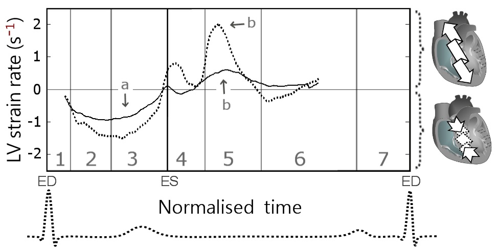
| Peak systolic longitudinal strain rate (s-1) | -1.3 ± 0.1 | -1.8 ± 0.2 | < 0.01 |
| Time to peak systolic longitudinal strain rate (% of end systole) | 44.6 ± 3.5 | 48.0 ± 3.2 | 0.60 |
| Peak diastolic longitudinal strain rate (s-1) | 1.1 ± 0.2 | 2.7 ± 0.1 | < 0.01 |
| Time to peak diastolic longitudinal strain rate (% of end systole) | 147.8 ± 2.5 | 134.4 ± 4.2 | 0.02 |
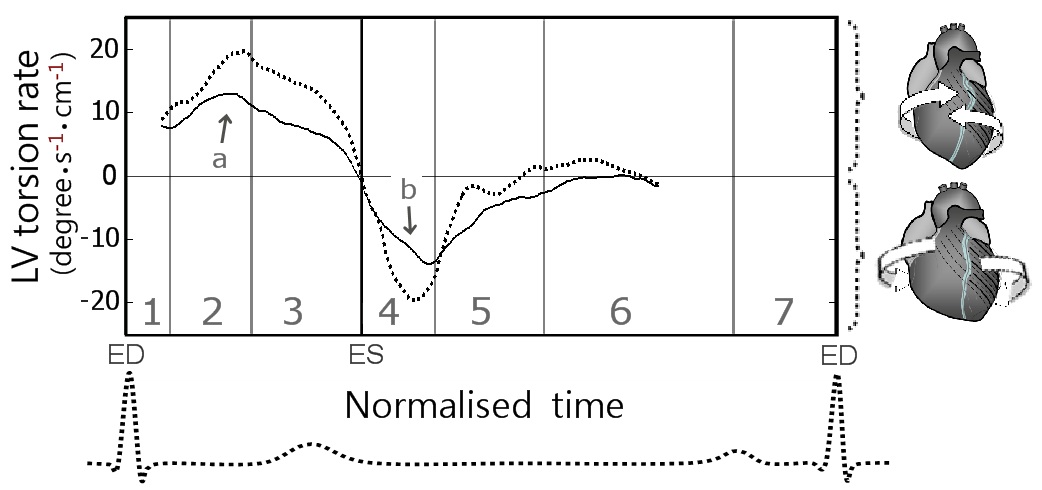
Figure 13: Global LV torsion rate during a cardiac cycle.
DISCUSSION
Reduced radial ventricular wall motion in CAD
Alterations in left ventricular rotation in CAD
The delay in LV apical untwisting in CAD subjects, made the clockwise rotation of the LV apex (Figure 5C, wave h, solid line) coincide at least partially with the clockwise rotation of the LV base (Figure 5A, wave f, solid line). This concordance in motion direction of the LV apex with the massive LV base may explain the much higher peak clockwise velocities at the LV apex (and even mid-ventricle) recorded in patients with CAD (Table 2 and Figure 5C, wave h, solid line). The altered rotational pattern of the LV apex might also explain the higher peak counter-clockwise velocities at the LV base (despite lower peak clockwise values) recorded in CAD patients. During the first half of isovolumetric relaxation, the LV apex in healthy subjects was rotating in a clockwise direction (Figure 5C, wave d, dotted line), which was opposite to the rotation of the LV base (Figure 5A, wave e, dotted line). In CAD patients, however, the LV apex was still rotating counter-clockwise during the first half of isovolumetric relaxation, the velocity trace showing negative values (Figure 5C, solid line). Thus, in healthy controls, the LV base and apex were rotating in opposite directions, whilst in CAD patients the counter-clockwise rotational recoil of the LV base encountered little or no resistance from the LV apex, resulting in higher peak values. These findings demonstrate how an altered rotational pattern of the ventricular apex can directly affect the rotational motion of the LV base. Significant alterations of LV rotational pattern were also noted during the phase of rapid ventricular filling, when the LV apex was rotating clockwise in CAD patients (Figure 5C, wave h) and counter-clockwise in healthy controls (Figure 5C, wave e). Most of these alterations of rotational pattern are expected to directly affect the ventricular physiology and LV filling. Correlative studies involving ventricular hemodynamics may shed new light into these mechanisms.
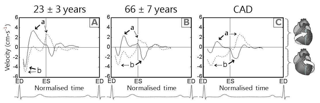
To provide a better understanding of the altered pattern of rotational motion of the LV apex and base against each other, we compared the circumferential velocity graphs with those obtained in a younger age group (healthy controls 23 ± 3 years old from an unrelated study [17]) (Figure 15). The graphs showed successive changes, with initial alterations of the rotational motions of the left ventricle in older age group and subsequent progressive loss of the undulating pattern of ventricular twisting in patients with CAD. Of particular note is that the peak counter-clockwise velocity at the LV base in younger subjects was represented by the initial wave of counter-clockwise rotation of the entire ventricle at the commencement of systole (Figure 15A, solid line, wave b), whilst in the older age group, as well as in patients with CAD it was represented by a recoil wave of ventricular untwisting in diastole (Figure 15B and C, solid line, wave b).
Pronounced alterations in ventricular longitudinal motion in CAD
Since the ventricular apex shows little motion along the longitudinal axis, due to concomitant LV shortening/twisting in systole and elongation/untwisting in diastole, the greatest difference in longitudinal motion can be expected at the LV base. In this study, the peak longitudinal velocities at the LV base were approximately two times lower in CAD patients compared with the values registered in healthy controls, representing the most significant difference between the two groups (Figure 9A, wave b). These findings were confirmed by similar differences in longitudinal strain rates (Table 4 and Figure 14). Our results are concordant with the findings reported in patients with acute myocardial ischemia, indicating reduced global longitudinal strain as the single most powerful marker of manifest left ventricular hemodynamic deterioration in the acute phase of myocardial infarction [36]. After the acute phase, longitudinal strain also proved an important predictor for segmental and global LV function improvement [37]. Furthermore, peak systolic longitudinal strain at rest was reported useful in predicting the presence of left main and three vessel coronary artery disease even before the development of regional wall motion abnormalities [38].
We also believe the findings would complement our previous studies [16,17], providing a broader understanding of underlying changes in left ventricular wall motion in elderly individuals, patients with coronary artery disease and subsequent ventricular remodeling following revascularization.
Study limitations and perspectives
CONCLUSION
The study revealed significant differences in radial, rotational and longitudinal LV motions as well as changes within myocardial layers in patients with CAD. The changes were more pronounced towards the LV apex, the sub-endocardial myocardium being affected to a greater extent. An altered pattern of ventricular rotational motion was also observed. The greatest difference between the two groups was noted in the longitudinal recoil motion of the left ventricle during diastole. Consequently, peak diastolic longitudinal velocity at the LV base and peak diastolic longitudinal strain rate might represent the most sensitive parameters in assessing global LV contractility. Further studies are needed in single and multivessel disease to determine whether these parameters provide important diagnostic and prognostic information for patients suffering from CAD.
ACKNOWLEDGEMENTS
This research was supported by British Heart Foundation grant number RG/07/004/22659.
REFERENCES
- Moen CA, Salminen PR, Grong K, Matre K (2011) Left ventricular strain, rotation, and torsion as markers of acute myocardial ischemia. Am J Physiol Heart Circ Physiol 300: 2142-2154.
- Mahenthiran J, Das MK, Bhakta D, Ghumman W, Feigenbaum H, et al. (2006) Prognostic importance of wall motion abnormalities in patients with ischemic cardiomyopathy and an implantable cardioverter-defibrillator. Am J Cardiol 98: 1301-1306.
- Sanderson JE, Wang M, Yu CM (2004) Tissue Doppler imaging for predicting outcome in patients with cardiovascular disease. Curr Opin Cardiol 19: 458-463.
- Safford RE, Bove AA (1987) Prediction of coronary artery disease by left ventricular regional wall motion abnormalities in patients with stenosis of the aortic valve. Br Heart J 57: 237-241.
- Yuda S, Fang ZY, Marwick TH (2003) Association of severe coronary stenosis with subclinical left ventricular dysfunction in the absence of infarction. J Am Soc Echocardiogr 16: 1163-1170.
- Launbjerg J, Berning J, Fruergaard P, Eliasen P, Borch-Johnsen K, et al. (1992) Risk stratification after acute myocardial infarction by means of echocardiographic wall motion scoring and Killip classification. Cardiology 80: 375-381.
- Carluccio E, Tommasi S, Bentivoglio M, Buccolieri M, Prosciutti L, et al. (2000) Usefulness of the severity and extent of wall motion abnormalities as prognostic markers of an adverse outcome after a first myocardial infarction treated with thrombolytic therapy. Am J Cardiol 85: 411-415.
- Kjøller E, Kober L, Jørgensen S, Torp-Pedersen C (2000) Short and long term prognostic importance of regional dyskinesia versus akinesia in acute myocardial infarction. Heart 87: 410-414.
- Herz SL, Hasegawa T, Makaryus AN, Parker KM, Homma S, et al. (2010) Quantitative three-dimensional wall motion analysis predicts ischemic region size and location. Ann Biomed Eng 38: 1367-1376.
- Li XC, Jin FL, Jing C, Xiao Q, Liu Y, et al. (2012) Predictive value of left ventricular remodeling by area strain based on three-dimensional wall-motion tracking after PCI in patients with recent NSTEMI. Ultrasound Med Biol 38: 1491-1501.
- Ishizu T, Seo Y, Baba M, Machino T, Higuchi H, et al. (2011) Impaired subendocardial wall thickening and post-systolic shortening are signs of critical myocardial ischemia in patients with flow-limiting coronary stenosis. Circ J 75: 1934-1941.
- Hauser AM, Gangadharan V, Ramos RG, Gordon S, Timmis GC (1985) Sequence of mechanical, electrocardiographic and clinical effects of repeated coronary artery occlusion in human beings: echocardiographic observations during coronary angioplasty. J Am Coll Cardiol 5: 193-197.
- Hoffmann R, Altiok E, Nowak B, Heussen N, Kühl H, et al. (2002) Strain rate measurement by doppler echocardiography allows improved assessment of myocardial viability inpatients with depressed left ventricular function. J Am Coll Cardiol 39: 443-449.
- Grabka M, Wita K, Tabor Z, Paraniak-Gieszczyk B, Chmurawa J, et al. (2013) Prediction of infarct size by speckle tracking echocardiography in patients with anterior myocardial infarction. Coron Artery Dis 24: 127-134.
- Yang J, Liu X, Jiang G, Chen Y, Zhang Y, et al. (2012) Two-dimensional strain technique to detect the function of coronary collateral circulation. Coron Artery Dis 23: 188-194.
- Codreanu I, Pegg TJ, Selvanayagam JB, Robson MD, Rider OJ, et al. (2011) Details of left ventricular remodeling and the mechanism of paradoxical ventricular septal motion after coronary artery bypass graft surgery. J Invasive Cardiol 23: 276-282.
- Codreanu I, Pegg TJ, Selvanayagam JB, Robson MD, Rider OJ, et al. (2014) Normal values of regional and global myocardial wall motion in young and elderly individuals using navigator gated tissue phase mapping. Age (Dordr) 36: 231-241.
- Jung B, Föll D, Böttler P, Petersen S, Hennig J, et al. (2006) Detailed analysis of myocardial motion in volunteers and patients using high-temporal-resolution MR tissue phase mapping. J Magn Reson Imaging 24: 1033-1039.
- Jung B, Markl M, Föll D, Hennig J (2006) Investigating myocardial motion by MRI using tissue phase mapping. Eur J Cardiothorac Surg 29: 150-157.
- Codreanu I, Robson MD, Golding SJ, Jung BA, Clarke K, et al. (2010) Longitudinally and circumferentially directed movements of the left ventricle studied by cardiovascular magnetic resonance phase contrast velocity mapping. J Cardiovasc Magn Reson 12: 48.
- Codreanu I, Robson MD, Rider OJ, Pegg TJ, Jung BA, et al. (2011) Chasing the reflected wave back into the heart: a new hypothesis while the jury is still out. Vasc Health Risk Manag 7: 365-373.
- Codreanu I, Robson MD, Rider OJ, Pegg TJ, Dasanu CA, et al. (2013) Effects of ventricular insertion sites on rotational motion of left ventricular segments studied by cardiac MR. Br J Radiol 86: 20130326.
- Codreanu I, Robson MD, Rider OJ, Pegg TJ, Dasanu CA, et al. (2014) Details of left ventricular radial wall motion supporting the ventricular theory of the third heart sound obtained by cardiac MR. Br J Radiol 17: 20130780.
- Cerqueira MD, Weissman NJ, Dilsizian V, Jacobs AK, Kaul S, et al. (2002) Standardized myocardial segmentation and nomenclature for tomographic imaging of the heart: a statement for healthcare professionals from the Cardiac Imaging Committee of the Council on Clinical Cardiology of the American Heart Association. Circulation 105: 539-542.
- Ishii K, Suyama T, Imai M, Maenaka M, Yamanaka A, et al. (2009) Abnormal regional left ventricular systolic and diastolic function in patients with coronary artery disease undergoing percutaneous coronary intervention: clinical significance of post-ischemic diastolic stunning. J Am Coll Cardiol 54: 1589-1597.
- Hu N, Sabey KH, Curtis HR, Hoang N, Dowdle SB, et al. (2012) Magnetic Resonance Imaging (MRI) assessment of ventricular remodeling after myocardial infarction in rabbits. Comp Med 62: 116-123.
- Oh BH, Volpini M, Kambayashi M, Murata K, et al. (1992) Myocardial function and transmural blood flow during coronary venous retroperfusion in pigs. Circulation 86: 1265-1279.
- Torry RJ, Myers JH, Adler AL, Liut CL, Gallagher KP (1991) Effects of nontransmural ischemia on inner and outer wall thickening in the canine left ventricle. Am Heart J 122: 1292-1299.
- Reimer KA, Lowe JE, Rasmussen MM, Jennings RB (1977) The wavefront phenomenon of ischemic cell death. 1. Myocardial infarct size vs duration of coronary occlusion in dogs. Circulation 56: 786-794.
- Vatner SF (1980) Correlation between acute reductions in myocardial blood flow and function in conscious dogs. Circ Res 47: 201-207.
- Geer JC, Crago CA, Little WC, Gardner LL, Bishop SP (1980) Subendocardial ischemic myocardial lesions associated with severe coronary atherosclerosis. Am J Pathol 98: 663-680.
- Stork A, Müllerleile K, Bansmann PM, Koops A, Meinertz T, et al. (2007) [Patterns of delayed-enhancement in MRI of ischemic and non-ischemic cardiomyopathies]. Rofo 179: 21-30.
- Kroeker CA, Tyberg JV, Beyar R (1995) Effects of ischemia on left ventricular apex rotation. An experimental study in anesthetized dogs. Circulation 92: 3539-3548.
- Götte MJ, Germans T, Rüssel IK, Zwanenburg JJ, Marcus JT, et al. (2006) Myocardial strain and torsion quantified by cardiovascular magnetic resonance tissue tagging: studies in normal and impaired left ventricular function. J Am Coll Cardiol 48: 2002-2011.
- Henein MY, Gibson DG (1999) Long axis function in disease. Heart 81: 229-231.
- Ersbøll M, Valeur N, Mogensen UM, Andersen MJ, Møller JE, et al. (2012) Relationship between left ventricular longitudinal deformation and clinical heart failure during admission for acute myocardial infarction: a two-dimensional speckle-tracking study. J Am Soc Echocardiogr 25: 1280-1289.
- Abate E, Hoogslag GE, Antoni ML, Nucifora G, Delgado V, et al. (2012) Value of three-dimensional speckle-tracking longitudinal strain for predicting improvement of left ventricular function after acute myocardial infarction. Am J Cardiol 110: 961-967.
- Choi JO, Cho SW, Song YB, Cho SJ, Song BG, et al. (2009) Longitudinal 2D strain at rest predicts the presence of left main and three vessel coronary artery disease in patients without regional wall motion abnormality. Eur J Echocardiogr 10: 695-701.
- Bijnens B, Claus P, Weidemann F, Strotmann J, Sutherland GR (2007) Investigating cardiac function using motion and deformation analysis in the setting of coronary artery disease. Circulation 116: 2453-2464
- Urheim S, Edvardsen T, Torp H, Angelsen B, Smiseth OA (2000) Myocardial strain by Doppler echocardiography. Validation of a new method to quantify regional myocardial function. Circulation 102: 1158-1164.
- Kramer CM, Rogers WJ, Theobald TM, Power TP, Petruolo S, et al. (1996) Remote noninfarcted region dysfunction soon after first anterior myocardial infarction. A magnetic resonance tagging study. Circulation 94: 660-666.
- Götte MJ, van Rossum AC, Twisk JWR, Kuijer JPA, Marcus JT, et al. (2001) Quantification of regional contractile function after infarction: strain analysis superior to wall thickening analysis in discriminating infarct from remote myocardium. J Am Coll Cardiol 37: 808-817.
- Jurcut R, Pappas CJ, Masci PG, Herbots L, Szulik M, et al. (2008) Detection of regional myocardial dysfunction in patients with acute myocardial infarction using velocity vector imaging. J Am Soc Echocardiogr 21: 879-886.
- Berti M, Ghizzoni G, Gualeni A, Cantamessa P, Oneglia C (2012) Electrocardiographic pattern combined with echocardiographic wall motion abnormalities in stress related cardiomyopathies: clinical and pathophysiological insights. Arch Cardiol Mex 82: 22-30.
Citation: Codreanu I, Pegg TJ, Selvanayagam JB, Robson MD, Rider OJ, et al. (2015) Comprehensive Assessment of Left Ventricular Wall Motion Abnormalities in Coronary Artery Disease Using Cardiac Magnetic Resonance. J Cardiol Stud Res 2: 006.
Copyright: © 2015 Ion Codreanu, et al. This is an open-access article distributed under the terms of the Creative Commons Attribution License, which permits unrestricted use, distribution, and reproduction in any medium, provided the original author and source are credited.