Fractal Aspects of Epidemic Spread
*Corresponding Author(s):
Airton DeppmanInstituto De Fisica, Universidade De São Paulo, Brazil
Email:deppman@usp.br
Abstract
The main properties of a fractal model to describe the epidemic spread of diseases are discussed. The most important features of the epidemic process that leads to the conclusion of an underlying fractal structure are analyzed, and the meaning of the parameters of the model are investigated. It is shown that the existence of a fractal mechanism in the epidemic evolution leads to a simple relation between time interval for the epidemic spread and the population size. It is shown that the contamination rate varies with the population size. The relevant differences between the SIR model and the fractal model are discussed.
Keywords
SARS-COV-2 virus; Contamination
INTRODUCTION
The pandemic spread of the SARS-COV-2 virus alerted the world for the necessity to take immediate polices to avoid the fast spread of dangerous viruses that can cause a large number of deaths. The crises caused by that disease evidenced that we still do not have a system of alerts that is good enough to prevent fast contamination through the different regions. The facilities that allow the easy and fast displacement of people also ensure the mechanisms for the spread of diseases.
The most widely used model for epidemic evolution is the SIR model [1,2], that describes the time evolution of three classes of individuals: susceptibles, infected and recovered. The SIR model results in an exponential increase of the epidemic disease, but several analyses evidenced that a power-law behaviour would describe better the observed data [3,4]. If the functions that describe the time evolution of each class are the susceptible, S(t), the infected, I(t) and the removed, R(t), and the total population, given by the sum of individuals in each of those classes, is considered constant in the time scale of the epidemic contamination, the SIR model gives a set of three coupled differential equations:
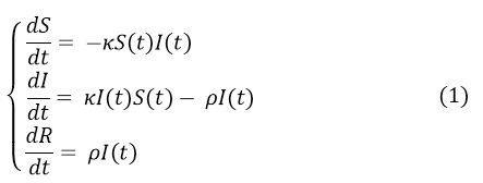 Where ρ and κ refer respectively to the removal rate of infected people and to the probability per unit of time that one infected subject will transmit the disease to a susceptible one.
While this approach can give a good description of the way contamination increases with time in a city, it is not enough to describe the spread of viruses in a very large population nor the spread of the virus in a network of interconnected cities, as we will see below. In general, virus contamination happens when there is close contact between the infected person and the susceptible one. Hence, one cannot consider that people in a large city have equal probability to meet any other person in the city, and the same holds for people located in different cities. The social behaviour in a city usually evolves to allow frequent contact of a person with a very small group of individuals, while most of the population will remain with no contact with that person [5,6].
The fact that social contact is structured by small groups is a universal feature of urban life and has consequences that can be observed in several analyses of socioeconomic behaviour [7-11]. One of the most striking features that emerge is the power-law distributions that are commonly found in the analyses. An intriguing result is that the exponent of the power-law seems to have a universal value, which is independent of country, culture or stage of development of the region analyzed [12,13]. The hypothesis of fractal structures underlying the behaviour of people in an urban environment is used more and more often to explain these observations [14,15].
Fractal structures appear whenever a system presents two distinguishing features: it is scale-free and it has an internal structure [16]. These two aspects lead to self-similarity, a remarkable aspect of fractals. From the geometrical figures to the biological system, going through physical systems and socioeconomic activity, fractals seem to be everywhere [14]. Recently, the fractal structure has been associated with Tsallis non-extensive statistics [17], with the non-additive index, q, being completely determined by the fractal parameters [18,19]. On the other hand, the Quantum Field Theory that is the prototype for three of the four known interaction in nature, the Yang-Mills Field Theory, points to the possibility of formation of fractal structures in all systems described by those interactions [20,21]. This result can explain why fractals are so common in natural systems.
On the other hand, the properties that ensure the emergence of fractal structures in the socioeconomic aspects of life in urban areas are still to be determined. The evidence for those fractal structures, as mentioned above, comes from the observed power-laws with an universal exponent. This power-law was found in the SARS-COV-2 disease pandemic, and a model for describing it in terms of the fractal structure was proposed [22]. We will investigate in details some of the characteristics of this model. It must be mentioned that in the case of SARS-COV-2, the fractal structures may be related to the aspect of the virus surface [23]. The non-linear spreading dynamics of diseases is studied in many works, e.g., Refs. [24-26].
In the fractal model developed in Ref. [22] the epidemic evolution is described by a set of two coupled differential equations, since
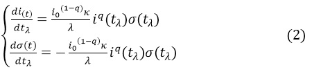
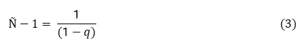
The main difference concerning the SIR equations (1) is the power q in the infected population that incorporates a feature of the Tsallis non-extensive statistics [17]. The meaning of the parameter q is the following: according to the model presented in [22], a large population is formed by a number of smaller groups, called agents, and the disease is transmitted by contact among the agents. Due to the fractal structure assumed in the model, each agent is formed by a number N˜ of other agents, with N˜ related to q by
The solution to the coupled equations are:
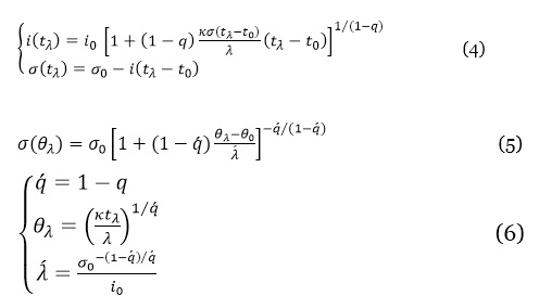
An approximate analytical solution for σ(t) can be obtained, resulting in With Therefore, the susceptible population follows a negative q-exponential function of the modified time variable, θ. Observe that the non-extensive distributions according to Tsallis statistics appear here as a consequence of the fractal structure. Different methods to include those distributions in the description of the epidemic spread were used [27].
Some clarifications about the meaning of the equations above are in order. Initially, important to observe that the power-law obtained for both infected and susceptible populations is a common feature of systems governed by fractal mechanisms, but it is not exclusively related to fractals since, as mentioned above, a fractal needs a power-law and an internal structure. The parameter λ plays the important role of the scale of the system, and therefore defines the hierarchy level of the fractal structure that is relevant for the description of the system. In the discussion below we will restrict ourselves to the number of infected described by the function i(tλ), but the same aspects are present also in the susceptible population, σ(tλ). The parameter tλ indicates that the time interval for the epidemic spread depends on the number of agents in each group. This dependence will be investigated below.
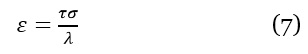
Observe that the quantity is a scale free variable in the fractal model proposed in Ref. [22]. Here ε embodies the main features of the fractal system: scale invariance and hierarchical structure. In the context of epidemic spread it represents the probability of contamination per direct contact between agents. When the population σ changes to σ'= aσ, the agent size changes from λ to λ'= aλ. If τ is independent of the scale, then ε is also scale independent.
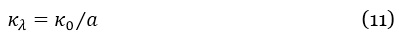
In many practical cases some scale is adopted as fixed, say λ=λo. For epidemic analysis the infected population is usually given by number of individuals, then λo=1. In this case,
we have:
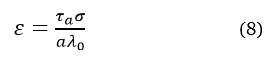
Since the epidemic dependence with the population σ is a power-law, as evidenced in data analyses, we can conclude from the expression above that τa/a is independent of the scale parameter, a, therefore τa=aτo. We can express the contamination in terms of a rate of transmission, κ, defined by τ=κλ(tλ−toλ), where to λ is the instant when the first infected agent appears in the group of σ individuals. In these terms we obtain
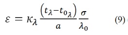 The interval tλ-toλ is the relevant time for the contamination of the group of size λ.
The time interval can be related to its counterpart at the scale λo by a function t (λ/λo, t), which we assume continuous and differentiable. A remark about the notation: t(., .) is a function of two variables and one of them is t, the time scale of epidemic spread in groups of size λo, while the symbol to is used to refer to the initial time of contamination for the group. For a=λ/λo varying in a limited range, and since the time for contamination is roughly proportional to the size of the group, we can write t(λ/λo, to)=a(t-to), where t and to are measured in the time scale compatible with λo. Therefore, in this time scale we have
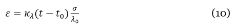
The assumption that ε is scale free results in the relation
where κo is the contamination rate at the scale λo, and represents the contamination per unit time, once the unit time and the scale of the agents are fixed. This result still implies in a scale-free spreading dynamics, since the variable ε remains independent of the scale.
The data analyses of SARS-COV-2, however, provide enlightening information about the way the spread of the COVID-19 disease took place in different regions of the world [22]. The fact that a power-law behaviour is observed means that the scale invariance is broken, so ε will be a linear function of the population σ. From the discussion made above, one can see that it will happen only if, for fixed λ=λo, the product κλ(tλ-to) will be independent of the scale of the population σ. There are two possibilities for it: the time span for contamination is independent of the size of the group, what seems to be contrary to the observations; the infection rate κ is independent of the size of the group. Here the second hypothesis is adopted.
If one assumes that the infection rate is independent of the size of the population in the group of infection, the Eq. 11 is not valid and must be replaced by κλ=κo. If follows from Eqs. (10) and (4) that the infected population increases as:
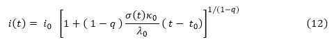
resulting in the power-law behavior of the distribution, as far as the time interval t-to is small enough to allow the population σ(t) be considered approximately constant.
The essential aspect to obtain the power-law behaviour is the fact that the rate of infection, κ, is independent of the scale. This is an interesting and unexpected result that deserves some additional comments. Observe that in Eq. (12) the number of agents is kept constant, since q is constant. The same holds for the scale λo and the time-scale, represented by a single time variable, t. The natural question that arises is: what happens if we change the scale of the groups, using a scale λ that is proportional to σ instead of λo? This aspect of the fractal epidemic process will be investigated below. Notice that:
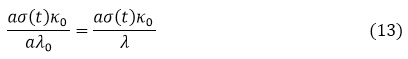
so, the infection rate will be given by κλ=aκ is the correct rate for groups of people with scale λ. If we assume that λo=1, that is, the scale refers to one single individual, then we can understand the meaning of κλ in the following way. When we change the scale, the agent of contact is not the individual, but a group with a number λ of individuals. The rate of infection among groups at that scale is λ times that for the infection among individuals, κo.
While this conclusion can seem to be intuitive, it unveils one the most important differences between the fractal description and the SIR-like models: here we keep the number of possible contacts inside a group constant, as given by q, and the argument of the power-law function changes according to the population size. In the SIR model, on the contrary, the number of ways the virus can be transmitted increases, and eventually goes to infinity. In fact, when q→1, the power-law behaviour we obtain here approaches the exponential behaviour of the SIR model. This difference can be traced down to the non-additivity of the entropy in the Tsallis statistics, which is closely related to the fractal structures [16]. In the case of epidemic spread, it is clear that the reason to obtain a power-law stems from the fact that, despite the large population that one can consider to be susceptible to infection, the number of ways one infected individual can transmit the disease is limited to the number of individuals in its close-contact group represented by the parameter q.
In conclusion, the meaning of the parameters that appear in the fractal model of epidemic spread is studied. The relation between the infection rate and the size of the population is obtained. Also, a discussion about the main differences between the fractal approach and the SIR approach is performed, and the important role played by the parameter q is analyzed.
ACKNOWLEDGMENTS
This work was supported by the Conselho Nacional de Desenvolvimento Científico e Tecnol´ogico (CNPq-Brazil), and by FAPESP under Grant No. 2016/17612-7.
REFERENCES
- Kermack WO, McKendrick AG (1927) A Contribution to the Mathematical Theory of Epidemics. Proceedings of the Royal Society of London A: Mathematical, Physical and Engineering Sciences 115: 700-721.
- Murray JD (2002) Mathematical biology. An Introduction. 3rd ed. Interdisciplinary Applied Mathematics.
- Komarova NL, Schang LM, Wodarz D (2020) Patterns of the COVID-19pandemic spread around the world: Exponential versus power laws. J R Soc Interface17: 20200518.
- Blasius B (2020) Power-law distribution in the number of confirmed covid-19 cases. Chaos 30: 093123.
- Batty M (2014) The New Science of Cities, MIT Press, Cambridge, MA.
- Batty M (2008) The Size, Scale, and Shape of Cities. Science 319: 769-771.
- Batty M (2014) “Cities and Complexity”, MIT Press, Cambridge MA.
- Schlapfer M, Bettencourt LMA, Grauwin S, Raschke M, Claxton R, et al. (2014) The Scaling of Human Interactions with City Size. Journal of the Royal Society Interface 11: 20130789.
- Bettencourt L, West G (2010) A unified theory of urban living. Nature 467: 912-913.
- Netto VM, Brigatti E, Meirelles J, Rebeiro F, Pace B, et al. (2018) Cities, from Information to Interaction. Entropy 20: 834.
- Bettencourt LMA, Lobo J, Strumsky D, West GB (2010) Urban Scaling and Its Deviations: Revealing the Structure of Wealth, Innovation and Crime across Cities. PLoS ONE 5: e13541.
- https://www.scientificamerican.com/article/bigger-cities-do-more-with-less/
- Bettencourt LMA, Lobo J, Helbing D, Kuhnert C, West GB (2007) Growth, innovation, scaling, and the paceof life in cities. The National Academy of Sciences of the USA 17: 7301-7306.
- https://link.springer.com/article/10.1007/s40823-019-00047-3
- Batty M, Longley P (1994) Fractal Cities: A Geometry of Form and Function, Academic Press, Cambridge, MA.
- https://onlinelibrary.wiley.com/doi/abs/10.1002/esp.3290080415
- Tsallis C (1988) Nonextensive physics: A possible connection between generalized statistical mechanics and quantum groups. Physics Letters A 195: 329-334.
- Deppman A (2016) Thermodynamics with fractal structure, Tsallis statistics, and hadrons. Phys Rev D 93: 054001.
- Deppman A, Frederico T, Megias E, Menezes DP (2018) Fractal Structure and Non-Extensive Statistics. Entropy 20: 633.
- Deppman A, Megias E, Menezes DP (2020) Fractals, nonextensive statistics, and QCD. Phys Rev D 101: 034019.
- Deppman A, Megias E, Menezes DP (2020) Fractal Structures of Yang-Mills Fields and Non-Extensive Statistics: Applications to High Energy Physics. Physics 2: 455-480.
- Abbasi M, Bollini AL, Castillo JLB, Deppman A, Guidio JP, et al. (2020) Fractal signatures of the COVID-19 spread. Chaos, Solitons & Fractals 140: 110119.
- Padhy S, Dimri VP (2020) Apparent scaling of virus surface roughness-An example from the pandemic SARS-nCoV. Physica D. Nonlinear Phenomena 414: 132704.
- Mohammad M, Trounev A (2020) On the dynamical modeling of COVID-19 involving Atangana–Baleanu fractional derivative and based on Daubechies framelet simulations. Chaos, Solitons & Fractals 140: 110171.
- Machado JAT, Ma J (2020) Nonlinear dynamics of COVID-19 pandemic: Modeling, control, and future perspectives. Nonlinear Dyn 101: 1525.
- Ribeiro HV, Sunahara AS, Sutton J, Perc M, Hanley QS (2020) City size and the spreading of COVID-19 in Brazil. PLoS ONE 15: e0239699.
- Tsallis C, Tirnakly U (2020) Predicting COVID-19 Peaks Around the World. Front Phys 29: 217.
Citation: Policarpo JMP, Meirelles AD, Ramos AAGF, Deppman A (2020) Fractal Aspects of Epidemic Spread. J Clin Immunol Immunother 6: 052.
Copyright: © 2020 Josué Mendes Pinheiro Policarpo, et al. This is an open-access article distributed under the terms of the Creative Commons Attribution License, which permits unrestricted use, distribution, and reproduction in any medium, provided the original author and source are credited.