Identification of Bio-Components Influencing Wheat Yields: Application of Spatial Regression Model

Wheat enjoys a special place among food products. This is because of the wide adaptability of cultivation under different climatic conditions, ease of cultivation, possibility of long-term maintenance, high nutritional value, and ability to be consumed in different forms. In addition, wheat has higher nutritional value in terms of proteins, carbohydrates, fats, minerals and vitamins than other food items [1]. In the world as a whole, it is the strategic product. Its annual production is 660 million tons, which supplies almost 20% of energy and 25% of protein needs of the world’s population [2]. 

Despite varied climatic conditions throughout the country, wheat is cultivated in almost all parts of Iran as a staple food. Iranian farmers allocate about 55% of the total cultivated area to this crop, i.e. 5 to 6 million hectares every year [3]. On the consumption side, Iranians’ average consumption of wheat is 2.5times than that in the world. A typical Iranian would consume about 167.6kg of wheat per year as against the average world consumption is only 67.1kgper year [4]. This indicates the importance of this product in agricultural sector as well as for consumers in Iran [5]. 

In spite of wheat’s importance in terms of area and consumption pattern, its yields are relatively very low. According to the statistics of Food and Agriculture Organization [4], Iran ranks 85^th in terms of wheat yield in 2013. Figure 1 shows the yield of Iran’s wheat production in comparison to four leading countries (Germany, Iceland, Netherlands and New Zealand). As it can be seen in this figure, the mean yield of the leading countries is about 8-9 tons ha^-1 while in Iran, the wheat yield only averages about 2 tons ha^-1 during the 1990-2013 period. This indicates that Iran has failed to keep pace with other similar nations in wheat productivity despite the growth of technology and efficiency in agricultural sector. Other nations have shown a steady increase in yield whereas Iran’s yields have become stagnant. 

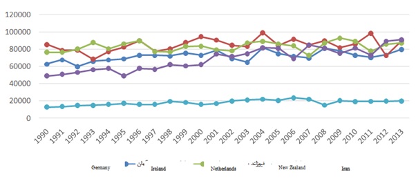Figure 1: Comparing the yield of wheat production in Iran with four top countries in terms of yield (kg per hectare); Source: Food and Agriculture Organization [4]. 

Increasing consumption patterns and stagnant production have led to Iran’s dependence on imports of wheat (Figure 2). As it can be seen, Iran has been dependent on imported wheat in all the studied years except with a few exceptions. Improvement in Iranian wheat production is therefore, an important policy issue in the country. Since an investigation of factors affecting production of wheat and identification of factors that would lead to an improvement in its yield has not been undertaken, this study was undertaken. Results can play a key and important role in reducing Iran’s dependency on imports and move the country towards self-sufficiency and sustainability. 

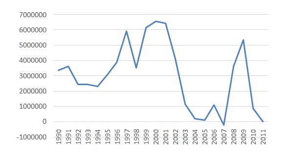Figure 2: Net import of wheat in Iran, 1990-2011. 

Khazaee and Hoshmand [6], used the data of 11 selected provinces to estimate the function of wheat production using ordinary least squares, random effects and Levinsohn and Petrin methods over the period 2000-2008. According to the results of the study, in ordinary least squares method, the coefficients estimated for water and fertilizer inputs were upward bias while capital inputs were estimated downward bias. The researchers concluded that in order to control bias due to the concurrency issues and selection, nonparametric methods should be used for modeling unobservable productivity shocks. Moradi Shahr-e Babak [7], selected an appropriate production function to evaluate the efficiency of almond producers in Sirjan and then, he estimated random frontier function and finally using duality theorem, he extracted frontier cost function from frontier production function and calculated the economic efficiency of beneficiaries. The results of the study by the researchers showed that the mean technical, allocative and economic efficiency of beneficiaries were 69, 64 and 44%, respectively. Raf’ati et al. [8], examined the technical efficiency, allocative and economic efficiency of cottontillers in Gorgan using parametric method. The data and information required for the study were collected among from 180 cottontillers in Gorganusing systematic random sampling method and in this regard, by estimating random frontier production function, the technical efficiency of cottontillers was calculated. Daneshvar et al. [9], compared partial and total productivity of production factors fortomatoin Khorasan Razaviusing Tornqvist-Theil index. The results of the study indicated that during the mentioned period, the index for input levels had an average growth rate of 0.022 in the tomato products. On the other hand, the output value had an annual average growth equal to 1.66 for the product. Salami and Nemati [10] evaluated the systemic risk of yield and factors affecting its intensity in apple products using spatial autoregressive model. The results revealed that apple-producing areas in the country are divided into two mountainous and foothill areas. The results of the additional spatial models also show that drought with one-year hiatus, the incidence of coldness in April, average temperature in July and August, total rainfall and the coefficient of rainfall variations per year encompass important climate variables affecting apple yield in Iran. Using spatial model, Wang and Zhang [11], showed that the yield of wheat, soya beans and corn are spatially dependent in different regions of the United States of America if the distance among regions is not more than 570 miles. Agnihotri et al. [12], examined the effect of the volume of irrigation water and its salinity on the yield and income of wheat in India using saltwater production function with quadratic function form. The results showed that 97% of yield variation was resulted by changes in quantity (size) and quality (salinity) of the irrigation water. The values of estimated coefficients show that the impact of water shortage is crucial on the yield variation of wheat compared to its salinity. Goni and Biba [13], investigated the factors affecting the yield of rice in Nigeria. For this purpose, the researcher has used a Cobb-Douglas functional form. The results showed that farmers have used all inputs except for workforce less than optimal level, which indicates mainly using inputs in a non-economic form. Kagabo et al. [14], examined soil erosion and yield of Rwanda’s agricultural products. The results of the study revealed that increasing the density of product cultivation in steep areas has increased soil erosion because of decline of fertility and productivity in the agricultural farms of these areas. Strikoik et al. [15], simulated the effect of low irrigation and the addition of nitrogen fertilizer on the yield of corn and productivity of water using Aqua Crop model in Delhi in 2009 and 2010.The results of the study showed that the above-mentioned model enjoyed a good accuracy in estimating the amount of biomass and weight of corn. The results also indicted that the accuracy of the model is decreased by increasing the level of stress so that the lowest accuracy was obtained in the treatment without adding fertilizer, while the highest accuracy was obtained in the treatment with the maximum low irrigation. 

The review of the studies conducted on the study subject indicates that so far, no comprehensive study has been done to estimate the biological production function of agricultural products within and outside the country. On the other hand, in the studies conducted for the estimation of production function, no spatial correlations have been considered in modeling by the researchers. Thus, this study sought to identify biological factors affecting the yield of wheat indryland farms in West Azerbaijan, Hamedan, Zanjan and Kurdistan in the form of spatial regression model.

Study areas and variables 

Data for this study were collected through field surveys in four dry land producing areas of Iran-West Azarbaijan, Zanjan, Hamedan and Kurdistan. Square shaped plots were established of 0.5 by 0.5M in dimension in each of these regions. In total each region has 90 such plots. In addition to removing some soil from these plots, data were recorded on slope, depth, slope direction and plowing. At the end of the crop season, wheat crop was harvested from these plots. The soil removed from the 360 plots (90 times 4 provinces) was sent to a laboratory for the quality of soil including attributes such as nitrogen, phosphorus, potassium absorbed by plant, and moisture at field capacity. The variables considered in this study included Yield of wheat (Y) as the dependent variable and the following independent variables, including soil Erosion (ERS), soil Depth (DE), Organic Materials of soil (OM), soil Moisture (FC), soil Nitrogen (N), soil Phosphorus (P) and soil Potassium (K). Figure 3 shows the location of the provinces in the study region.

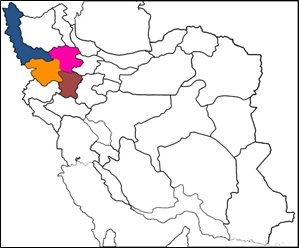Figure 3: The location of the areas under study.

 The study model 

Although farmers’ geographic and environmental conditions play a role in determining the yield of a crop, spatial variables related to location could also be relevant.  Since in this study, yields were estimated from four neighboring provinces, applying conventional econometrics methods is not recommended. In fact, under these situations, two types of effects would be present [16]: 

1. Spatial dependency among observations of the sample data in different locations and,
2. Spatial heterogeneity caused by the relationships or parameters of model, which change through movement on the coordinate plane with sample data.
3. Under this situation, conventional econometrics model, if used, would ignore both spatial dependency and heterogeneity. Furthermore, this would also violate the Gauss-Markov assumptions will be violated. In other words, by assuming the spatial dependence between data and movement among various samples, the relationship will change and the coefficients of a linear function will not be BLUE (Best Linear Unbiased Estimators). As a result, use of conventional econometric methods of estimation is recommended [8].

To deal with the above type of situation, another form of models has been developed--spatial models. In general, spatial models are divided into General Auto-regressive Spatial Model (SAC), Spatial auto-regressive Error Model (SEM), Mixed Auto-regressive Model (SAR) and Spatial Durbin Model (SDM) [16]. Each of these is described below. 

General Auto-regressive Spatial Model (SAC) 

General Auto-regressive Spatial Model (SAC) is the best model for spatial estimation [10], since both spatial error and lag are considered. The overall form of the model is shown as Equation (1) [16].

Where Y, X and W₁ and W₂ represent respectively, dependent variable, explanatory variable and spatial weight matrixes. The explanatory variables are as listed above--soil Erosion (ERS), soil Depth (DE), Organic Materials of soil (OM), soil Moisture (FC), soil Nitrogen (N), soil Phosphorus (P) and soil Potassium (K). Equation (1) can be expanded using a Cobb-Douglas functional form, as shown in Equation (2).

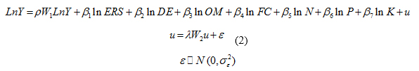
This equation has already been converted into a linear model using the logarithmic transformation. 

Auto-regressive model with Spatial Error Model (SEM) in errors 

In this model, one assumes that there is only spatial autocorrelation in the errors. In other words, in SEM, unlike S, . So, the overall shape of the model is shown as Equation (3) [16].

Including all the explanatory variable and using a Cobb-Douglas function linearized using the logarithmic transformation results in the model shown in Equation (4):

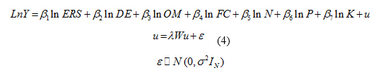
This model suggests that there is no direct correlation between the yields of wheat in four considered provinces; however, the correlation is performed through errors in neighboring regions. 

Mixed Auto-regressive Model (SAR) 

If in SAC model, is true, i.e. there is no spatial autocorrelation in errors in the model, the model has only spatial interruptions [17]. The overall form of the model is expressed as Equation (5).

The estimated empirical model is presented as Equation (6).

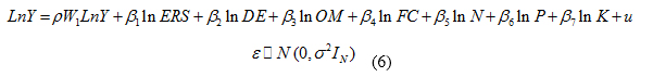
 In fact, the above equation shows that there is a direct correlation between the yields of wheat in four study provinces with no error taking place in neighboring areas.

Spatial Durbin Model (SDM) 

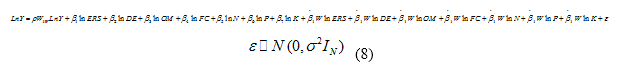
In this model, in addition to the lag of dependent variable in SAC and SAR models, the lag of independent variable is also added. This model is shown in Equation (7).

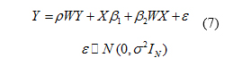
The empirical model of the study is presented in Equation (8).

 Determining the neighborhood matrix 

In order to estimate the spatial regression models, a neighborhood matrix is required. Generally speaking, this matrix is based on two features (1) adjacency and (2) distance. In this study, however, on account of nature of data collection, only adjacency was used. Given that the yield of wheat was collected in four provinces, the initial adjacency matrix was 4 by 4 for a single set of observation. Since there were 90sample cases in each province, the final matrix was of 360 by 360 dimension. The matrix takes a value zero for the main diagonal, one for other elements if two provinces are neighboring; otherwise, it is zero. The formed matrix is a symmetric matrix. Figure 4 shows the location of the provinces to form the adjacency matrix.

Figure 4: Definition of adjacency for the provinces under study.

According to the spatial adjacency, figure (4) of adjacency matrix is prepared as follows. As can be seen in figure 3, Area 1 is adjacent to Areas 2 and 3, Area 2is adjacent to Areas 1, 2 and 3 and Area 3 is adjacent to Areas 2, 3, 4 and Area 4is adjacent to Areas 2 and 3. Resultantly, value of 1 is used to show adjacency. For a single set of 4 plots, the resulting matrix is shown in Equation (9). This matrix is extended to all the 360 observations in the study and finally, resulting in a 360 by 360 matrix.

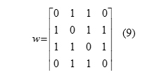
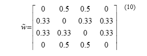
Finally, the standardized weight matrix is estimated by dividing the number elements by row total for each row, which is presented in equation (10) [16]. These values are used in the estimation of various spatial regression models presented above.

Application of a spatial regression model is advised only if some evidence of spatial dependency in data is found. In this study, this was evaluated using various tests described in this section. 

Moran test 

In the Moran test, its null hypothesis indicates lack of spatial effects in errors. If the null hypothesis is rejected, there are spatial effects in errors. In such circumstances, use of the LM test is recommended by Enslin [17]. The test is described in Equation (11).

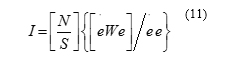
In the above equation, W and S is weight matrix, total components matrix of W and e vector for the components of error in the regression equation estimated by OLS, respectively.

LM-error test 

The LM-error test was developed by Beveridge [18]. The null hypothesis of this test shows the lack of spatial autocorrelation coefficient . If this hypothesis is rejected, the alternative hypothesis of spatial autocorrelation  is confirmed. If the null hypothesis of this test is rejected, SEM model should be estimated [19]. This test is shown in Equation (12) [17].

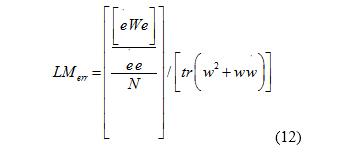
This statistics has a distribution with one degree of freedom. Part of this statistic is made up of the second square of Moran test and several other empirical studies [20,21]. In samples with low number of observations, Moran test has relatively better power than this test; however, in large samples, the performance of the two tests is identical.

LM-lag test 

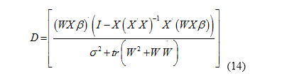
The null hypothesis of this test is that there is a lack of spatial autocorrelation in the model with the hypothesis that . If there is autocorrelation in the model   and the null hypothesis is rejected, the model with spatial lag should be estimated [19]. The test statistic is shown in Equation (13).

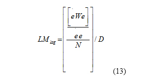
In Equation (13), D is defined as Equation (14).

The statistic of this test also has a distribution with one degrees of freedom. 

LM-lag-Robust and LM-error-Robust tests 

If the null hypothesis is rejected in both LM-lag and LM-error tests, in such conditions, the examination of Robust of both tests is recommended [22]. If the null hypothesis of Robust LM-error test based on the lack of spatial autocorrelation is rejected, spatial model with spatial autocorrelation should be used in errors. When the null hypothesis of Robust LM-lag test based on the lack of spatial autocorrelation is rejected, spatial model with spatial lag should be used [19]. 

In the event that the null hypothesis of both tests is rejected, the enlargement of two statistics will be evaluated so that if the statistic of Robust LM-error is larger, the spatial model with spatial correlation is estimated in errors and if the statistic of Robust LM-lag is also larger, the spatial model with spatial lag is selected for estimation. In case of different results, testing the common factor hypothesis must be considered. 

Common factor hypothesis test 

This test is used to select the Durbin model. If the null hypothesis of this test is rejected, Durbin model should be estimated since under the state of accepting the null hypothesis, using spatial model of dependency in errors is confirmed. Likelihood Ratio (LR) is the test statistic for this test [19].

Table 1 shows the results of different spatial models. In the first step, in order to determine the most appropriate model, the level of significance of the variables, diagnostic tests and criteria for goodness of fit in different models were examined. The results showed that the level of significance in all models, except SDM model with spatial lag explanatory variables, were similar. The results of Moran and Gary test confirmed spatial autocorrelation in errors. In the second step, because of these conditions, the LM-lag and LM-error tests were examined, their results revealed that both tests are significant at the level of 1%. As a result there was a need to assess two Robust-LM-lag and Robust-LM-error tests in order to select the most appropriate model. Research shows that the two tests were also significant at 1% level. In such circumstances, the magnitude of test statistics was considered. As shown in table 2 shows, the value of statistic Robust LM-error is greater than the statistic Robust LM-error where SEM model is better compared to SAR. On the other hand, given the significant level of the variables and indices of goodness of fit, R²_Buse and R^-2_Buse of the SAC model, it gives a better explanation situation than the selected SEM model. In addition, AIC and SC criteria of goodness of fit in SAC model were lower than the SEM, which confirmed the selection of SAC model.  

Table 1: Results of coefficients for the spatial regression models.

Source: research findings (* and **, *** are significant at 10%, 5% and 1%). 

Table 2: Test results determining spatial patterns.

Also testing the common factor hypothesis suggests that this test is significant at 1% level. Therefore, in such circumstances, the use of the spatial model of dependency in errors is rejected and the use of SDM model is confirmed.

Comparison between SAC and SDM models shows that the rates of R²_Buse  and R^-2_Buse in SAC model are 0.36 and 0.35, respectively and 0.70 and 0.69, respectively for SDM model that indicates that the SDM model provides a better power in explaining the variability in the yields of various regions. Moreover, the statistics of two criteria AIC and SC in SDM model is less than those in SAC model, which confirmed that the SDM model is superior.

Results of the estimated models indicate that variables such as soil Depth (DE), soil Moisture (FC), soil Phosphorus (P) level affect wheat yield in a positive manner, while soil Erosion (ERS), soil Potassium (K) and Nitrogen (N) affect wheat yields negatively [23]. The negative impact of potassium and nitrogen on wheat yield could be explained by the high amount of this nutrient that is found in the soil in the study region. In fact, soil potassium and nitrogen of most fields in the study regions was higher than the average of other fields. Three variables--nitrogen, potassium and organic matter were not found to be statistically significant. Depth and soil moisture have the greatest impact on wheat yield in rain fed areas. Soil moisture is a key component in the production process and germination and early plant establishment in the soil, followed by wheat growth depends on it. Thus, holding other variable constant, one percent increase in soil depth and soil moisture would increase wheat yield by as much as 0.59 and 0.25 percent. Phosphorus is the other key variable which has a significantly positive effect on the yield of wheat in the studied region. On the other hand, variables that exerted a negative effect on wheat yield included soil Erosion (ERS), with the coefficient of 0.22 and soil Nitrogen (N) and soil Potassium (K) with coefficients of 0.052 and 0.053, respectively. The high impact of soil erosion on the wheat yields indicates the deterring role of this variable and suggests avenue for increased wheat yields.

The growth of population is one of the main factors to bring about more demand for food in Iran (as well world over). To meet this demand, increased supply (availability) is necessary. Providing sufficient food to masses of people has always been one of the most important challenges for many countries, even more so for Iran. Wheat being a major staple food in Iran may deserve some credit in achieving this objective.  This study was undertaken to find the variables that affect yield of wheat in northwest part of Iran. This study was performed in West Azarbaijan, Zanjan, Hamedan and Kurdistan using the method of spatial regression. 

Of all the factors affecting wheat yields, biological components and natural characteristics of soil are important in the growth process of plants. Based on relative performance of various types of spatial regression models, the SDM model showed a better performance in explaining wheat yields in the study region. Relations among the study variables showed that soil depth, moisture at field capacity and soil phosphorus had a positive effect on the yield, while soil erosion, soil potassium and soil nitrogen had a negative effect. Among these variables, soil depth and moisture had the higher positive effect and soil erosion had the higher negative effect on the yield of wheat. Thus, according to the obtained results: 

• It is recommended to pay enough attention to various factors related to soil, especially soil depth and slope of cultivation, as well as loss of soil nutrient through erosion and over use of inorganic nutrients.
• It is recommended to provide favorable conditions for sustainable production of wheat in the country through the correct choice of crop varieties adapted to climatic conditions and potentials of areas.
• Given the importance of tillage on increasing the soil permeability for rainfall which provides suitable conditions for reducing runoff and water and wind erosion and improving soil moisture retention, using modern tools and methods can play a significant role in increasing the yield of wheat.
• It is recommended touse modern econometrics methods in conjunction with other conventional models to accomplish better results in future studies.

REFERENCES

- Heidari Kh, Cheraghi D (2004) Investigating the share of waste and smuggling of wheat in the food security of Iranian households, 1st national conference on prevention of waste of national resources, Tehran, Islamic Republic of Iran's Academy of Sciences.
- Khabis FH, Mousavi MB, Bakhtiari B, Aval MB (2014) The effects of rainfall on dryland wheat yield and water requirement satisfaction index at different time scales. Journal of Irrigation and Water Engineering 5: 1-13.
- Ehsani M, Khalidi H (2004) Identifying and improving the productivity of agricultural water to supply water and food security in the country, 11th Seminar of Iranian National Committee on Irrigation and Drainage in Iran.
- FAO (2013) FAO statistical book. FAO Statistics Divisions.
- Ahmadvand M, Najafpour Z (2007) Assessing the performance of guaranteed purchase policy of agricultural products using exchange relationship 65: 5-14.
- Khazaei J, Hoshmand M (2014) Non-parametric nonlinear control of productivity shocks in estimating the agricultural production function in the selected provinces of Iran (Case study: to estimate the wheat production function). Journal of Economics and Agricultural Development 28: 246-259.
- Moradi H (2001) Determining the yield of almond producers in Kerman (Case study: Sirjan), Investigations of agricultural economy 2: 117-132.
- Raf'ati M, Azarinfar Y, Barabari A, Kazemnejad M (2011) Examining the technical, allocative and economic performance of Golestan cotton using parametric methods (Case study: Gorgan), Agricultural Economics Research 1: 121-142.
- Daneshvar M, GolrizZiaee Z, Razavi H (2008) Evaluating the productivity of tomato in Khorasan Razavi, First National Congress of tomato production and processing technology, Mashhad, Iran.
- Salami H, Nemati M (2013) investigating the systemic risk of yield and factors affecting its intensity on apple in Iran: Use of spatial autoregressive model. Economy and agricultural development 4: 288-299.
- Holly Wang H, Zhang H (2003) On the possibility of a private crop insurance market: A spatial statistics approach.Journal of Risk and Insurance 70: 111-124.
- Agnihotri AK, Kumbhare PS, Rao KVGK, Sharma DP (1992) Econometric consideration for reuse of drainage effluent in wheat production. Agricultural water management22: 249-270.
- Goni M, Mohammed S, Baba BA (2007) Analysis of resource-use efficiency in rice production in the Lake Chad area of borno state, Nigeria. Journal of Sustainable Development in Agriculture and Environment3: 31-37.
- Kagabo DM, Stroosnijder L, Visser SM, Moore D (2013) Soil erosion, soil fertility and crop yield on slow-forming terraces in the highlands of Buberuka, Rwanda.Soil and tillage research 128: 23-29.
- Stricevic R, Dzeletovic Z, Djurovic N and Cosic M (2014) Global change biology bioenergy.
- LeSage JP (1999) The theory and practice of spatial econometrics. University of Toledo, Toledo, USA.
- Anselin L (2001) Rao's score test in spatial econometrics.Journal of statistical planning and inference 97: 113-139.
- Burridge P (1980) On the Cliff-Ord test for spatial autocorrelation among regression residuals.Geographical Analysis 4: 267-284.
- Osland L (2010) An application of spatial econometrics in relation to hedonic house price modeling.Journal of Real Estate Research 32: 289-320.
- Anselin L, Rey S (1991) Properties of tests for spatial dependence in linear regression models.Geographical analysis 23: 112-131.
- Anselin L, Florax RJ (1995) Small sample properties of tests for spatial dependence in regression models: Some further results. InNew directions in spatial econometrics. Springer Berlin Heidelberg, Berlin, Germany. Pg no: 21-74.
- Anselin L (1988) Spatial Econometrics: Methods and Models. Springer Science & Business Media, Berlin, Germany.
- Ghrbani M (2001) An economic analysis of soil erosion in Iran: the cost of water erosion, Ph.D. Thesis. University of Tehran, Enghelab Square, Iran.
Citation: Ghorbani M, Kulshreshtha S, Radmehr R, Dadrasmoghaddam A (2020) Identification of Bio-Components Influencing Wheat Yields: Application of Spatial Regression Model. J Agron Agri Sci 3: 022.
Copyright: © 2020 Mohammad Ghorbani, et al. This is an open-access article distributed under the terms of the Creative Commons Attribution License, which permits unrestricted use, distribution, and reproduction in any medium, provided the original author and source are credited.