Selection of Optimal Treatment Regimen for Individuals Using Multivariate Assessments during Clinical Follow-Up

In medical practice, doctors and patients will have to decide on the best treatment regimen to maximize treatment benefit. In some cases, it is a matter of “do or die”. Crucial as it is, the treatment selection criteria suffer from “the curse of dimensionality”, which means due to factors known and unknown, some patients have higher likelihood of cure after immediate surgery while others respond positively to less invasive treatments. To tackle the problem of uncertainty associated with treatment selection, statistic techniques such as causal inference studies are conventionally employed, despite the fact that causal effect is usually a constant rather than a function, hence a lack of predictive ability of covariates in evaluating individualized treatment selection of heterogeneous patients.

In the literature, two approaches and their hybrids made it possible to derive an optimal treatment rule. The first approach targets at predicting the average result difference of biomarkers in two comparison groups or multiple comparison groups. Notably, the average result difference is not a constant but a biomarker-dependent function, and these biomarkers may be single, multiple or even high-dimensional. For the selection of an optimal treatment regimen based on a single biomarker, Ma and Zhou [1] proposed a method using Covariate-Specific Treatment Effect (CSTE) curves, which was followed up by Han et al., [2] based on the cases where the outcome variables are binary. 

Guo et al., [3] extended their research to high-dimensional data which is cross-sectional rather than longitudinal, and failed to build statistical inference upon the situation when the data was obtained from actual treatments in multiple follow-ups and thus longitudinal. To advance their study, Gao [4] investigated the longitudinal data from repeated measurements of outcomes of a single biomarker by using the spline-based Generalised Estimating Equation (GEE) method to estimate the CSTE curve, and identified its asymptotic nature. Based on the asymptotic normality of CSTE curves, the confidence bands in the CSTE curves were constructed. The results of numerical simulation and case analysis show that the estimation of the CSTE curve and its confidence band proved the efficiency of the estimators.

In practical scenarios, longitudinal follow-up studies often involve multidimensional or high-dimensional covariates, attributable to the inclusion of multiple biomarkers or high-dimensional biomarkers. Based on this, an attempt was made to expend previous longitudinal single-biomarker studies to multiple biomarker ones, and corresponding CSTE curve estimation methods were presented. Regarding the parameter estimation of CSTE curves for high-dimensional longitudinal data, the Smoothly Clipped Absolute Deviation (SCAD) penalty was employed, specifically, the penalised GEE (PGEE) method utilized by Wang et al., [5] to estimate the parameters. 

Despite being a robust strategy, the CSTE curves cannot generate optimal treatment policy without the estimation of confidence bands. Song [6] determined optimal treatment regimens via the Selection Influence Curve (SIC) and employed the bootstrap method to obtain the confidence band. Ma and Zhou [1] used the Resampling (RS) technique to construct the confidence bands for the CSTE curve with continuous response variables. Moreover, Zhou et al., [7] proved the asymptotic normality of the regression spline and applied the Hotelling Tube method to construct the confidence bands. Subsequently, Loader et al., [8] and Krivobokovaa et al., [9] followed a similar approach in constructing the confidence bands of the estimators. 

Han et al., [2] applied this method to construct the confidence band of the CSTE curve for cross-sectional data of single biomarker with binary outcome. Gao also applied it to construct confidence band of the CSTE curves with longitudinal single biomarkers, and Guo et al., constructed confidence bands of the CSTE curves using the Spline Back-Kernel (SKB) estimators. In this paper, we applied Hotelling Tube method to construct confidence band of the CSTE curves for longitudinal data of multiple biomarkers and high-dimensional biomarkers. 

This paper is organized as follows: 

In Section 2, we introduce the optimal treatment regimen selection method based on CSTE curves using multivariate and high-dimensional clinical follow-up data. Section 3 presents the simulation study, and a conclusion is given in Section 4.

Defining CSTE curve with multivariate clinical follow-up data 

Notations are given here for the sake of convenience in the following discussions.

We consider a sample of N subjects (i=1, 2,......,N), each of whom was observed for  times. Let  Y_ij (k) be the outcome variable of the j-th observation of the i-th individual receiving the k-th treatment regeimen, and the indicator variable W_ijl represents whether the i-th subject select the l-th treatment regimen in the j-th observation. A value of 1 indicates acceptance of the l-th treatment regimen, and 0, otherwise. (W_ij1,W_ij2,...,W_ijd) = W^T_ij indicates the d-th treatment regimen available for the j-th observation of the i-th subject. If there is only one treatment option available, each subject has a pair of potential outcomes in the j-th observation, denoted as ((Y_ij (0),Y_ij (1)). If the i-th subject is in the control group, then  is an unobservable latent variable and  is an observable variable. If the i-th subject is in the treatment group, then the opposite is true. Namely, Y_ij = W_ijY_ij (1) + (1-W_ij) is the measurable outcome variable of the i-th individual's j -th observation. X_ij represents that the covariate of the j-th measurement of the i-th subject is a vector, denoted as. X _ij = (X_ij1,X_ij2,...,X_ijp).

Underlying Hypothesis 1: Stable unit treatment value, which implies that subjects who receive treatments do not interfere with each other’s potential outcome, and for any concerned subject, each treatment corresponds to only one potential outcome.

Underlying Hypothesis 2: The ignorability assumption, denoted as, W⊥(Y(0),Y(1))|X, also known as the unconfoundedness assumption, was proposed by Rosenbaum and Rubin (1983), who observed that the treatment assignment is ignorable and does not depend on the potential outcome. 

Single treatment programs: Based on these hypotheses, the outcome variables in a single binary treatment program, W , are:

Y_ij = W_ijY_ij (1) + (1-W_ij) Y_ij (0)

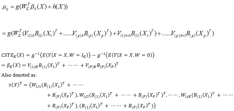
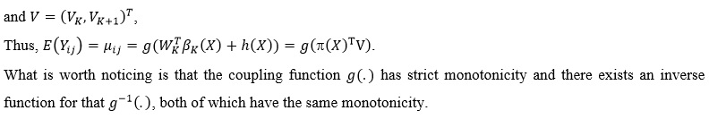
Let E (Y_ij), = μ_ij  hypothetically, g(.) is assumed to be a joint function with strict monotonicity, and there exists an inverse function denoted by 

g^-1(.), μ_ij = g (W^T_ij β(X _ij) + h (X _ij)).

The CSTE curve for a longitudinal univariate single-treatment regimen is assumed to be (Gao, 2020):

CSTE(x) = g^-1(E(Y|X = x, W = 1)) - g^-1(E(Y|X = x, W = 0))

However, the above definition was based on single covariate, when there are multiple covariates, which is often the case in practice, we redefine longitudinal multivariate CSTE function as:

CSTE(x) = g^-1(E(Y|X = x, W = 1)) - g^-1(E(Y|X = x, W = 0))

Here, X is a vector.

Multiple treatment programs

Gao (2020) assumed that the CSTE curves for the k-th treatment option of longitudinal univariate are:

CSTE(x) = g^-1(E(Y|X = x, W = I_K)) - g^-1(E(Y|X = x, W = 0))

In the above equation, the I_K is a vector with the k-th element being 1 and the remaining elements being 0. The monotonicity of  can be obtained g^-1(.) from the monotonicity of g^-1(.). However, the above definition is only based on one covariant and become unapplicable in case of multiple covariates; Accordingly, we provide a definition of multivariate variables. Assuming the CSTE curves for the k-th treatment regimen of the longitudinal multivariate are:

CSTE_K(X) = g^-1(E(Y|X = X, W = I_K)) - g^-1(E(Y|X = X, W = 0))

Here, X is a vector.

CSTE curve estimation based on multivariate clinical follow-up data

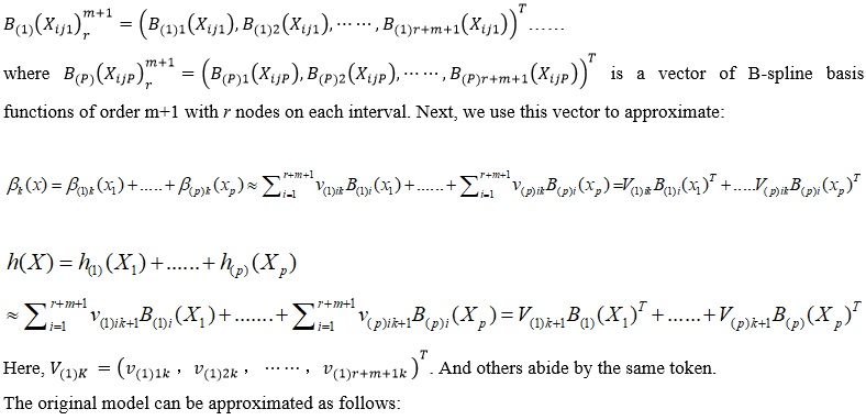
Estimation of CSTE function: B-spline function approximation 

Applying the B-spline function to approximate our estimation of the CSTE function leads to the following assumptions:

Assumption 1: X _ij = (X_ij1,X_ij2,...,X_ijp) , in which the domain of each component is a compact set.

Assumption 2:The distance between r nodes of B-spline basis function with order m+1 on the interval [a, b] is equal.

Assumption 3: The CSTE curve CSTE_K(X) is m+1 order continuous in the defined domain.

Assumption 4: The presence of a C > 0 maker = CN^1/(2m+1) 

Suppose the biological indicators of the subjects are denoted as X , then the value for each component is respectively : [a₁, b₁] ......[a_p, b_p]:

Model parameter estimation

CSTE estimation of asymptotic normality

The asymptotic normality of the estimation of longitudinal univariate CSTE curves was proven by Gao (2020). On this basis, under the above assumptions in this paper, it was not difficult to obtain the following properties of CSTE_K :

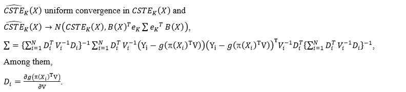
Next, we apply Hotelling Tube method to construct the confidence band for the simultaneous promotion of CSTE curves over the entire domain of definition.

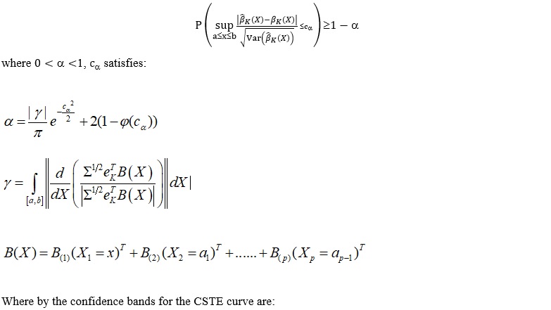
Construction of confidence bands for the generalization of CSTE estimation

In fact, if there are two covariates, the geometric meaning of the CSTE function is no longer a curve but a surface. For the convenience of research and to visually demonstrate how to select the optimal treatment regimen as different covariates change, when we examine a certain covariate, we might as well take other covariates as a certain constant in the definition domain. For example, if there are two covariates, one is discrete as X₁ with values of 1 and 2, and the other is continuous as X₂. We set the value of X1 as 1, CSTE (X) = CSTE (X₁ = 1, X₂) remains a curve, and the treatment regimen is selected based on the change in the value of the biological indicators X₂.

Similarly, when X₁ has value of 2, CSTE (X) = CSTE (X₁ = 2, X₂) remains a curve, and the treatment regimen is selected based on the change in the value of the biological indicator X₂.

At the same time, as is well-known, continuous variables can be discretised, especially in actual treatment. For the normal range of some biological indicators, we may as well mark the value as 1, and mark the non-normal range as 2. Therefore, the continuous variable X₂ can be discretized according to the practical significance of its value. Assuming that the values are 1 and 2, respectively, we get CSTE (X) = CSTE (X₁, X₂  = 1) and CSTE (X) = CSTE (X₁, X₂  = 2) seperately, and make the choice of treatment according to the change of the value of the biological indicator X₁. For multiple covariates, the method is analogous. In the following discussion, we assume that the variable which is not a constant in the multi-dimensional CSTE curve estimation is X₁, with the value of  x and the domain of definition is [a,b].

Based on the assumptions of this paper and a sufficiently large sample size, it was not difficult to obtain the following conclusions by applying Hotelling Tube method:

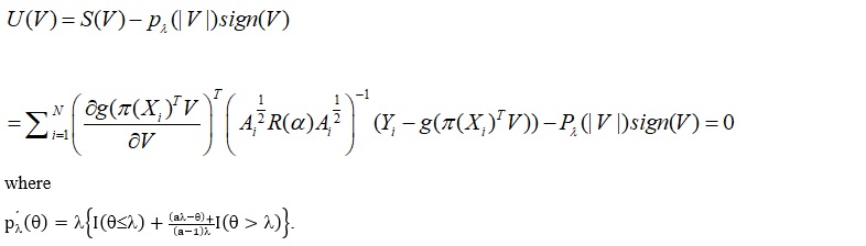
CSTE curve estimation for high-dimensional clinical follow-up data

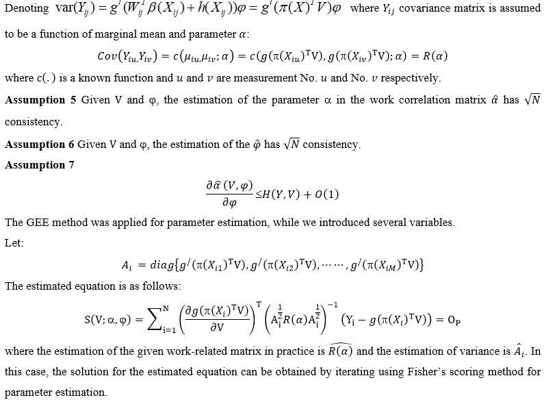
In this section, we examined the CSTE curve estimation in the case of high-dimensional data. The CSTE estimation is still in accordance with the above discussed B-spline function approximation. In addition, we resolved the high-dimensional problem using the SCAD penalty in the parameter estimation, that is, we applied the PGEE method in the parameter estimation:

In this section, we investigate the feasibility and large sample property of our proposed method via simulated datasets.

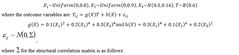
Simulation study of the multivariate clinical follow-up data 

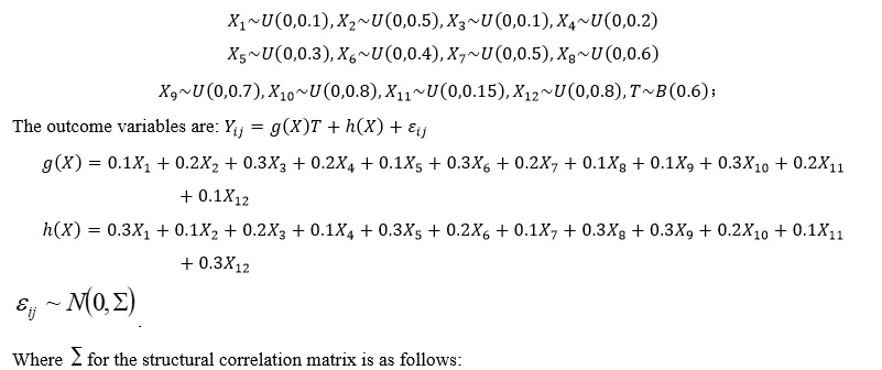
300 datasets were randomly generated in order to examine the three covariates, then, the specific covariates and the treatment program indicator variables were generated as follows:

The evaluation of the goodness-of-fit of the GEE adopts the QIC and QICC criteria based on the quasi-likelihood function, as the likelihood function is no longer applicable to the GEE. Here, QIC was used to select the correlation matrix under a given model, while QICC was used to select the model under a given correlation matrix. For both indices, the smaller the value, the better the corresponding structure or model.

Factoring in the estimation method of the correlation matrix to three settings, namely, independent structure, unspecified structure and autocorrelation structure when generating simulation data. 300 experiments were conducted for each setting to observe the estimation of the parameters and the CSTE curves. In the experiments, the smoothing parameters, m and r, were determined by cross-validation, and the QICs estimated by different combinations of m and r  were compared to select the smoothing parameter combination that minimises the QIC. table 1 shows the mean square error (MSE) and mean absolute error (MAE) in the CSTE curve estimation.

Table 1: Estimates of the CSTE function for Simulation 1: Multivariate clinical follow-up and confidence bands.

Abbreviations: CP, coverage probabilities; MAE, mean absolute error; MSE, mean square error.

It can be seen from table 1 that as the sample size increases, the MSE and MAE decrease, the length of the confidence interval decreases, and the coverage rate increases. Whether the correlation matrix type is correctly specified or not, both MSE and MAE are relatively small, and they are the smallest when the correlation matrix type is correctly specified. 

In figure 1, we discretised variables X₁ and X₃, If both ≤ 0.5, they take the value of 1, otherwise, 0. We consider the case where X₁ takes the value of 1 and X₃ takes the value of 0. By examining the CSTE curves with the change of X₂, it can be seen that the curves are all > 0 within the range of the X₂ values, so the treatment regimen should be selected.

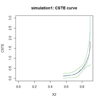 Figure 1: Simulation 1: CSTE curve.

Simulation study of high-dimensional clinical follow-up data

300 datasets were randomly generated in order to examine the three covariates, then, the specific covariates and the treatment program indicator variables were generated as follows:

As can be seen from table 2, MSE and MAE are decreasing as the sample size increases, and both MSE and MAE are smaller with or without the correctly specified correlation matrix type, with the smallest in the correctly specified case.

Table 2: Estimates of the CSTE function for Simulation 2: high-dimensional clinical follow-up.

Abbreviations: MAE, mean absolute error; MSE, mean square error.

In this paper, we proposed the estimation method for multivariate CSTE curves in clinical follow-up by taking account of the definition of longitudinal univariate CSTE curves and using GEE and spline function estimation with an additive model. The confidential band we constructed may grant a higher percentage of success in therapeutical decisions. As for high-dimensional CSTE curves, PGEE is exploited to model the selection impact curve. Simulation studies show that as the sample size increases, the estimated values approximate the true values, the length of the confidence intervals decreases while the coverage rate increases, indicating good large-sample properties.

Ethics approval and consent to participate 

This research complied with national policies and regulations. 

Consent for publication 

We declare that there are no conflicts of interest regarding the publication of this manuscript. 

Availability of data and materials 

The data that support the fundings of this research are available from the corresponding author upon reasonable request. 

Competing interests 

The authors declare that they have no competing interests. 

Funding 

This research was supported by the National Social Science Foundation of China (Grants No. 18FTJ003), the Academic Research Projects of Beijing Union University (No. ZKZD202306), and the Research Project on Water Price Pricing Model of Shanxi Large Water Network Project. 

Author’s Contribution 

Except for the corresponding author, the other authors are ranked according to their contribution.(Corresponding Author:Yi Danhui,First Author:Han Feng,Second Author:Zhang Lin lin,Co - Fourth Author:Zhang Jingsheng and Han Kaishan). 

Acknowledgement 

We would like to express our deepest gratitude to our families. They have always been our strongest supporters, and their encouragement and companionship are the driving force of our academic pursuit. In addition, we are lucky to have each other in the research team to work closely and learn from each other.

1. Ma Y, Zhou XH (2017) Treatment selection in a randomized clinical trial via covariate-specific treatment effect curves. Statistical Methods in Medical Research 26: 124-141.
2. Han K, Zhou X-H, Liu B (2017) CSTE Curve for Selection the Optimal Treatment When Outcome Is Binary. Scientia Sinica Mathematica 47: 497-514.
3. Wenchuan G, Hua ZX, Shujie M (2021) Estimation of Optimal Individualized Treatment Rules Using a Covariate-Specific Treatment Effect Curve with High-Dimensional Covariates. Journal of the American Statistical Association 116: 309-321.
4. Yanxia G (2020) Using CSTE curve to select the optimal scheme under longitudinal data. East China Normal University, China.
5. Lan W, Jianhui Z, Annie Q (2012) Penalized generalized estimating equations for high-dimensional longitudinal data analysis. Biometrics 68: 353-3
6. Song X, Pepe MS (2004) Evaluating markers for selecting a patient's treatment. Biometrics 60: 874-83.
7. Zhou S, Shen X, Wolfe DA (1998) Local asymptotics for regression splines and confidence regions. The annals of statistics 26: 1760-1782.
8. Loader C, Sun J (2012) Robustness of Tube Formula Based Confidence Bands. Journal of Computational and Graphical Statistics 6: 242-250.
9. Krivobokova T, Kneib T, Claeskens G (2010) Simultaneous Confidence Bands for Penalized Spline Estimators. Journal of the American Statistical Association 105: 852-863.