2030 Ozone Source Attribution from Nox Emission Reduction Modeling Study

Planning strategies to attain future year compliance with the National Ambient Air Quality Standards (NAAQS) rely on the use of air quality models to predict changes in air quality. The decline in ozone levels has slowed since 2010, and attainment is predicted to be decades into the future [1-4]. Ozone is created by a reaction in the atmosphere of Nitrogen Oxide (NO_x) and Volatile Organic Compound (VOC) emissions and certain favorable meteorological conditions [5,6]. The design of effective emission control strategies requires an understanding of the contributions of different categories of emission sources to the pollutant of interest. For secondary pollutants, such as ozone and secondary fine Particulate Matter (PM2.5), Photochemical Grid Models (PGMs) are typically used to characterize source contributions because they can simulate the physical and chemical processes that affect dispersion and reaction of air pollutants in the atmosphere [7]. These contributions can be determined either by Brute Force Methods (BFM), in which emissions from the source of interest are changed, typically by zeroing out emissions from that source, and the resulting concentrations are subtracted from the base case concentrations, or by source apportionment tools that are available in current PGMs. Examples of the latter are the Ozone Source Apportionment Technology (OSAT) in the Comprehensive Air Quality Model with Extensions, (CAMx) [8] and the Integrated Source Apportionment Method (ISAM) [9,10] in the U.S. EPA Community Multiscale Air Quality (CMAQ) Model [11-13]. The Direct Decoupled Method (DDM) [14] is another tool available in CAMx or CMAQ to conduct source sensitivity analysis. 

Previous studies by the authors used source apportionment and source sensitivity methods to characterize source contributions and to calculate source sensitivities [15,16]. Those earlier studies provided insight on the contributions of major anthropogenic source categories to ozone levels in different regions of the United States and provided information on relative changes (e.g., a 20% reduction) in precursor emissions from a source category on ozone concentrations. Those studies found the ozone reduction percentage trends for a source category when using High-Order Decoupled Direct Method (HDDM) [17] or BFM were correlated to almost the same percentage of the base NO_x emission. In other words, the studies found the emission source categories which have higher amount of NO_x emissions have a higher ozone reduction impact. This does not provide a way to evaluate the influence of precursor reduction to ozone reduction except for the percentage of NO_x emissions with these methods. 

The major scientific motivation for this study was to evaluate the ozone change based on a fixed amount of NO_x emission reduction for each source category. This would highlight unique conditions for each area, such as meteorological and geographical conditions. This paper describes the use of the brute force method approach in a hypothetical study to determine the impact of reducing future year NO_x emissions by a specified amount from each of the major source categories on future year ozone design values. Since the same absolute amount of NO_x reductions were applied to each source category over a defined area, this provided a fairer comparison of benefits from the reduction, as compared to relative changes that may overemphasize the benefits of source categories that have much higher emissions than other categories. The BFM can be used for studying ozone changes predicted after precursor reductions using a percentage or a fixed amount. So, the BFM was determined to be more appropriate for this type of fixed-amount precursor reduction analysis than the other source apportionment or source sensitivity methods. 

The analysis was conducted for ozone attainment and non-attainment areas. For non-attainment areas, the South Coast Air Basin (SoCAB) and the San Joaquin Valley (SJV) in California were selected. The state of Maryland was chosen because it had changed from an ozone non-attainment to attainment area. NO_x emissions from the various source categories were reduced by nearly 15 tons per day. While the selection of the reduction amount in this study was based on the smallest total NO_x emissions from the different source categories, i.e. 14.9 TPD in Maryland from light duty gasoline vehicles, the reduction amount is also comparable with the NO_x reductions of 15 TPD sought by the South Coast Air Quality Management District, the regulatory agency for the SoCAB, via additional incentive funding [18] in its contingency measure plan to attain the 1997 8-hour ozone standard in 2023. The hypothetical study described in this paper considers the impact of 15 TPD NO_x reductions from each of the 5 major anthropogenic source categories: Light Duty Gasoline Vehicles (LDGV), Heavy Duty Diesel Vehicles (HDDV), off road sources, area sources, and point sources.

The objective of the study described here was to quantify absolute changes in future year 8-hour average ozone design values as a result of absolute reductions of 14.9 TPD of NO_x emissions from each of the five major anthropogenic source categories. Future year ozone design values with and without the emission reductions were calculated at all monitors of interest in the two California air basins, SoCAB and SJV, and at monitors of interest in Maryland. The BFM was employed by conducting multiple PGM simulations with emissions from one source category reduced at a time. The same PGM and modeling databases used in the previous source apportionment and source sensitivity studies [16,19] were used for this study. Those studies used the CAMx model [20] with the CB6r4 chemical mechanism and the EPA 2011 v6.2 modeling platform [21]. As part of the previous studies, a model performance evaluation was conducted for the base year 2011 and the model performance was found to be satisfactory [16]. Since the same model and modeling platform were used in the current study, the performance evaluation is not discussed here. 

CAMx modeling was conducted on two smaller subdomain of the large CONUS (continental US) domain. The first domain, figure 1a covered Maryland and parts of the surrounding states, the other domain was in the western US and covered the two California air basins: figure 1b for the SJV area, and figure 1c for the SoCAB. A five-day spin-up period was used for the subdomain future year simulations. Boundary conditions for the subdomain modeling were developed using full CONUS simulations for the base year 2011, and the future year 2030, from previous studies [16,19]. For the western US NO_x reduction simulations, NO_x emissions in the two California air basins were reduced proportionally to achieve a combined NOx emission reduction of 14.9 TPD for each source category. For the Maryland domain simulations, NOx emissions in Maryland were reduced by 14.9 TPD for each source category. The study did not consider reductions in VOC (including CO) emissions. NO_x emissions in the SoCAB, SJV, and Maryland were reduced for the following 5 anthropogenic source categories (1 category at a time): LDGV; HDDV; off-road mobile; point sources; and other area sources. Cell mask files for each air basin [19] were used to designate model grid cells corresponding to the air basins for the emission reduction scenarios. Scaling factors based on the total reduction amount were used to reduce NO_x emissions in each model grid cell. As discussed above, for the western subdomain the scaling factors were based on the combined SoCAB and SJV emissions, i.e., 14.9 TPD of NO_x emissions were removed from the combined emissions in the same proportion as their base emissions. Next, the scaled emissions were merged with the remaining modeling inventory sources to develop the model-ready files for the ten Future Year Emission Scenarios (five NO_x scenarios for the California subdomain and five NO_x scenarios for the Maryland subdomain). Because the two California regions (SJV and SoCAB) were simulated in a single run for each source category NO_x reduction, there may be a small impact of NO_x reductions in one region (e.g., SJV) influencing ozone design value changes in the other region. 

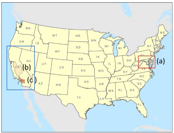
Figure 1: Locations of subdomains within the CONUS domain: (a) Maryland, (b) SJV, (c) SoCAB.

Table 1 summarizes the NO_x emissions in the SoCAB, SJV, and Maryland areas by source category for the 2030 Base Case, scaling factors used to reduce the emissions by 14.9 TPD, and the resulting NO_x emissions for each source category for the BFM scenario simulations. The LDGV emissions in Maryland are reduced by 100% because the base 2030 LDGV emissions are 14.9 TPD. Also, the combined SoCAB and SJV NO_x emissions are reduced by 14.9 TPD keeping the relative proportion of the emissions from each air basin the same as in the base 2030 emissions. For example, the LDGV scaling factor is shown in equation 1.  

1-(14.9/(3.92+12.68)) = 0.1030                                                        (1)

Thus, the scaling factors for SJV and SoCAB are identical. 

Table 1: NO_x emissions in by source category: 2030 Base Case, scaling factor, BFM Scenario.

Figure 2 shows the spatial distribution of the reduction in NO_x emissions for the SoCAB.

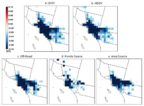Figure 2 : Spatial distributions of NO_x emission reductions (reduction scenario – base) for SoCAB. NO_x reduction source categories are shown from left to right, top row: LDGV, HDDV; bottom row: off-road, area and point. 

Future year ozone design values for the different emission reduction scenarios were calculated at monitoring locations in the three different regions, using EPA’s Modeled Attainment Test Software (MATS) [22]. The design value calculations, described below, require base case results for both the base year (2011) and future year. The base case results for 2011 and 2030 were available from the previous studies [16,19], so this work focused on the emission reduction scenarios for each source category for the future year. 

The MATS processing followed EPA’s guidance on calculating the future year design values. The use of MATS to calculate future year design values is described in detail in Collet et al., 2018b. Briefly, the modeling results are used in a relative sense to scale observed site?specific base year (2011) 8-hour ozone Design Value Concentrations (DVCs) based on the relative changes in the modeled 8-hour ozone concentrations between the current year and the future year. Future year ozone design values are calculated by using the relative changes in model results between the base year and future year and applying these changes, referred to as Relative Response Factors (RRFs), to the base year observation-based design value. The RRF is the ratio of the future year modeled concentration predicted near a monitor (averaged over multiple days) to the base year modeled concentration predicted near the monitor (averaged over the same days). 

Table 2 provides a list of monitors in the state of Maryland and the two California air basins where future year ozone design values were calculated using MATS and the CAMx modeling results. The monitors in table 2 are the same as in the previous studies [16,19]. 

Table 2: List of monitoring sites in the South Coast Air Basin (SoCAB) the San Joaquin Valley (SJV) and Maryland. All monitoring sites were considered in the BFM study. The 2030 ozone design value (DVF).

Differences in future year ozone design values due to the NO_x reductions are difficult to discern using absolute values. Thus, figure 3 shows the changes in future year ozone design values for the five BFM scenarios considered in this study. The changes are shown as Future Year Scenario (2030) Future Year Base (2030). A negative change implies a reduction in ozone and a positive change implies an increase in ozone resulting from the NO_x emission reductions. Figure 3a depicts the Maryland results, figure 3b represents results from SJV, and figure 3c shows the results for the SoCAB. For Maryland, figure 3a, all monitors show reductions in ozone design values resulting from the NO_x emission reductions from any of the 5 anthropogenic source categories. This is consistent with the understanding that the region is NO_x limited and is thus sensitive to NO_x reductions and is also consistent with the isopleth (EKMA) diagrams for Maryland [19]. The ozone reductions are generally less than 1 ppb, with the exception of the Edgewood monitor, where the reduction is nearly 1.6 ppb for a 15 TPD NO_x emissions reduction from off-road sources. Table 3 ranks the 5 source categories according to the ozone reductions resulting in Maryland from the 15 TPD NO_x reductions and also ranks the spatial distribution of the reductions in NO_x emissions. The NO_x reduction dispersion was ranked by determining the total number of 0.1 TPD squares shown as an example in figure 2. The category with the largest number of dark squares was considered to have the most dispersion or largest area for the NO_x reductions, and the smallest number of dark squares was considered to have the least dispersion or smallest area for NO_x reductions. As shown in table 3, the rankings for the two quantities are identical, indicating that the source categories with larger areas of NO_x reductions have the largest impacts on ozone reductions and vice-versa. Off-road sources have the highest rank for both the NO_x reduction dispersion and the ozone reduction, while area sources have the lowest rank.

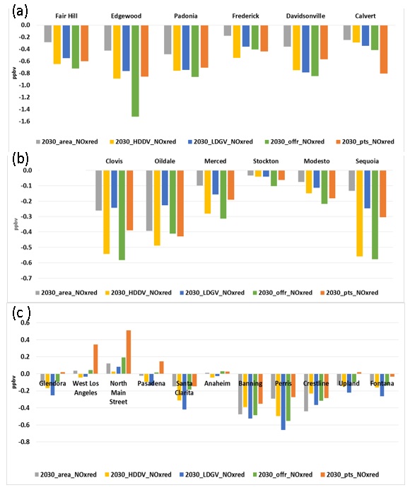Figure 3: Changes (scenario – base) in future year ozone design values due to 14.9 TPD NO_x emission reductions in (a) Maryland, (b) SJV, and (c) SoCAB.

The results for the SJV monitors shown in Figure 3b, are qualitatively similar to the Maryland results. All the monitors show reductions in future a year ozone design value resulting from the NOx emission reductions supporting that the SJV region is also NO_x limited. The emission reductions have a negligible effect on design values at the San Francisco monitor, which is generally upwind of the SJV. Ozone reductions at the SJV monitors are also small, ranging from less than 0.1 ppb to a maximum of about 0.6 ppb. These reductions are smaller than at the Maryland monitors. Possible reasons for the differences are 1) only a fraction of the 15 TPD NO_x emission reduction is from sources in the SJV, since the 14.9 TPD reduction was applied to the combined SJV and SoCAB, and 2) results from previous ozone source apportionment studies show that boundary conditions are large contributors (40% to 50%) to ozone at many monitors in the SJV [16]. 

Table 3 shows the rankings of the NO_x reduction dispersion and the ozone reductions are identical for the SJV monitors, similar to the case of the Maryland monitors. Off-road sources have the highest rank in the SJV while area sources have the lowest rank (similar to the Maryland results). However, between these two extremes, there are some differences in the ranking of the other source categories. For example, point sources have the second largest effect on the Maryland monitors, while NO_x emissions from HDDVs have the second largest effect on the SJV monitors. In both regions, LDDV emissions have the second lowest effect on ozone design values. 

Table 3: Source rank in Maryland, and SJV for NO_x reduction dispersion and for ozone reduction (Figure 3).

Figure 3c shows the changes in future year ozone design values at the SoCAB monitors from the NO_x emission reductions from the five BFM scenarios. The results for the SoCAB monitors show more variability than the NO_x limited regions of Maryland and the SJV and can be grouped into three classes: monitors showing increases in ozone, monitors showing large decreases in ozone, and monitors showing small decreases in ozone. There are some increases in future year ozone design values at SoCAB monitors near Los Angeles, i.e., urban sites that are VOC-limited and less responsive to NO_x reductions. At these VOC-limited areas, reductions in NO_x emissions have an ozone increase. In contrast, at the downwind sites, such as Banning, the NO_x or VOC emission reductions result in decreases on ozone design values. This is consistent with the isopleth (EKMA) diagrams for SoCAB [19]. The decreases in ozone design values are generally higher for LDGV NO_x emissions than for HDDV emissions, possibly because reductions in SoCAB NO_x emissions from LDGVs are about 11 TPD, while the corresponding reductions from HDDVs are about 8 TPD, table 1. Table 4 presents the NO_x reduction dispersion and ozone reduction rankings for the SoCAB, and shows no obvious correlation between the two rankings as noted for both Maryland and the SJV. 

Table 4: Source rank in SoCAB for NO_x reduction dispersion (Figure 2) and for ozone changes (Figure 3).

The future year ozone isopleths (EKMA diagrams) [19] shown in figure 4, provide some insight into the results obtained in this study. While the EKMA diagrams do not differentiate among the emission reductions from different source categories, the diagrams show the responses to overall reductions in emissions. In the case of Maryland, which is NO_x-limited, the VOC vs NO_x contours in the isopleths show a nearly linear response to NO_x reductions and minimal or no response to VOC reductions. The difference in response to NO_x reductions between the various Maryland monitors is also explained by the isopleths. For example, the Frederick monitor shows a lower response than the Padonia monitor to the same amount of NO_x reductions, Figure 3a. The isopleth diagrams for the two monitors, Figure 4a also show the Frederick monitor requires a larger amount of NO_x reductions to achieve the same ozone reduction as the Padonia monitor. Similarly, the SJV is also NO_x limited and the isopleths show sensitivity to NO_x changes and negligible sensitivity to VOC changes. At two monitors in the SJV, Stockton and Merced, showing large differences in ozone responses to NO_x reductions, Figure 3b, have isopleths which show the Stockton monitor needs more NO_x reductions to achieve the same level of ozone reductions as at the Merced monitor. On the other hand, the EKMA diagrams for many of the SoCAB monitors show sensitivity to both NO_x and VOC changes, with some monitors in the urban areas (e.g., the Los Angeles monitor) having more sensitivity to VOC emissions than NO_x emissions and negative sensitivity to NO_x emissions at certain ozone levels. The source-targeted results for the SoCAB monitors are consistent with the isopleth diagrams from the previous work [19]. For example, the Fontana monitor has a lower response than the Banning monitor to the same amount of NO_x reductions, Figure 3c. The isopleth diagrams for the two monitors, Figure 4b, also shows the Fontana monitor requires a larger amount of NO_x reductions to achieve the same ozone reduction as the Banning monitor. The NO_x reduction difference between ozone isopleths when comparing Fontana and Banning can also explain the large and small decreases of ozone in SoCAB.

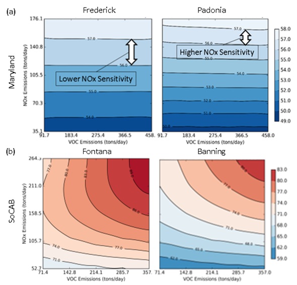
Figure 4: Ozone isopleths for monitors in (a) Maryland, (b) SoCAB.

This study used CAMx simulations and the BFM to simulate the effect of reducing 14.9 TPD NO_x emissions from a number of anthropogenic source categories on future year (2030) ozone design values at monitors of interest in the South Coast Air Basin (SoCAB) and San Joaquin Valley (SJV) in California and in the state of Maryland. Five major anthropogenic source categories were selected for the analysis: LDGV, HDDV, off-road mobile, point sources, and other area sources. The ranking of the source categories according to the ozone benefits achieved by reducing NO_x emissions by the same amount from each category are different by area and within the same area. The NO_x limited Maryland and SJV regions show some similarities in their ozone responses, with the most ozone reductions from off-road sources and the least reductions from other area sources. Reducing LDGV emissions has the second lowest ozone reductions in both regions. In the SoCAB, ozone increases at some VOC-limited locations when NO_x emissions are reduced, with reducing NO_x emissions from point sources resulting in the most ozone increase. At many downwind monitors in NO_x-limited areas of the SoCAB that showed decreases in ozone resulting from the emission reductions, LDGV NO_x reductions resulted in larger ozone decreases than the other categories for the same amount of emission reductions. However, LDGVs are the smallest NO_x emitters in California (and Maryland) due to enhanced regulations on NO_x emissions, and the 15 TPD reduction conducted in this hypothetical study represents nearly a 100% reduction in combined LDGV NO_x emissions in the SJV and SoCAB air basins and a 100% reduction in Maryland. Thus, it is difficult to expect further NO_x reduction from LDGV sources.

REFERENCES

- Bishop GA (2019) Three Decades of On-road Mobile Source Emissions Reductions in South Los Angeles. J Air & Waste Management Association 69: 967-976.
- US Environmental Protection Agency (2015) National Ambient Air Quality Standards for Ozone. Environmental Protection Agency (EPA), Washington DC, USA.
- Fujita EM, Campbell DE, Stockwell WR, Saunders E, Fitzgerald R, et al. (2016) Projected ozone trends and changes in the ozone-precursor relationship in the South Coast Air Basin in response to varying reductions of precursor emissions. J Air Waste Manage Assoc 66: 201-214.
- Parrish DD, Young LM, Newman MH, Aikin KC, Ryerson TB (2017) Ozone Design Values in Southern California's Air Basins: Temporal Evolution and U.S. Background Contribution. J Geophys Res Atmos 122: 166-111.
- Simon H, Wells B, Baker KR, Hubbell B (2016) Assessing Temporal and Spatial Patterns of Observed and Predicted Ozone in Multiple Urban Areas. Environ Health Persp 124: 1443-1452.
- Seinfeld JH, Pandis SN (1998) Atmospheric Chemistry and Physics from Air Pollution to Climate Change (3rdedn). Environmental Chemistry. Pg no: 1152.
- Zawacki M, Baker KR, Phillips S, Davidson K, Wolfe P (2018) Mobile source contributions to ambient ozone and particulate matter in 2025. Atmosp Sci 188: 129-141.
- Ramboll Environment and Health (2018) User’s Guide, Comprehensive Air Quality Model with Extensions (CAMx), version 6.50, California, USA.
- Kwok RHF, Napelenok SL, Baker KR (2013) Implementation and evaluation of PM2.5 source contribution analysis in a photochemical model. Atmos. Environ 80: 398-407.
- Kwok RHF, Baker KR, Napelenok SL, Tonnesen GS (2015) Photochemical grid model implementation and application of VOC, NOx and ozone source apportionment. Geosci Model Dev 8: 99-114.
- Byun D, Schere KL (2006) Review of the governing equations, computational algorithms, and other components of the Models-3 Community Multiscale Air Quality (CMAQ) modeling system. Appl Mech Rev 59: 51–77.
- Foley KM, Roselle SJ, Appel KW, Bhave PV, Pleim JE, et al. (2010) Incremental testing of the Community Multiscale Air Quality (CMAQ) modeling system version 4.7. Geosci Model Dev 3: 205-226.
- EPA (2019) CMAQv5.3 User's Guide, U.S. Environmental Protection Agency, Research Triangle Park, N.C, Washington DC, USA
- Dunker AM (1980) The response of an atmospheric re/action-transport model to changes in input function, Atmos. Environ 14: 671-679.
- Collet S, Kidokoro T, Karamchandani P, Shah T, Jung J (2017) Future-year ozone prediction for the United States using updated models and inputs. J Air & Waste Management Association 67: 938-948.
- Collet S, Kidokoro T, Karamchandani P, Jung J, Shah T (2018a) Future year ozone source attribution modeling study using CMAQ-ISAM. J Air & Waste Management Association 68: 1239-1247.
- Zhang W, Capps SL, Hu Y, Nenes A (2012) Development of the high-order decoupled direct method in three dimensions for particulate matter: enabling advanced sensitivity analysis in air quality models. Geosci Model Dev 5: 355-368.
- SCAQMD (2019) AQMP Advisory Group, Public Workshop documents, South Coast Air Quality Management District, Los Angeles, USA.
- Collet S, Kidokoro T, Karamchandani P, Shah T (2018b) Future-Year Ozone Isopleths for South Coast, San Joaquin Valley, and Maryland. Atmosphere 9: 354.
- Environ International Corp (2016) User’s Guide, Comprehensive Air Quality Model with Extensions (CAMx), version 6.40. Environ International Corp, Washington DC, USA.
- EPA (2011) 2011 Version 6 Air Emissions Modeling Platforms, Environmental Protection Agency, Washington DC, USA.
- EPA (2010) Modeled Attainment Test software, User’s Manual, U.S. Environmental Protection Agency, Washington DC, USA.
Citation: Collet S, Kidokoro T, Yamashita T, Karamchandani P, Shah T (2020) 2030 Ozone Source Attribution from Nox Emission Reduction Modeling Study. J Atmos Earth Sci 4: 017.
Copyright: © 2020 Susan Collet, et al. This is an open-access article distributed under the terms of the Creative Commons Attribution License, which permits unrestricted use, distribution, and reproduction in any medium, provided the original author and source are credited.