Calculating Global Temperature Anomalies using Three New Methods

HadCRUT4 [1-3] is one of the most widely used global temperature records and was originally adopted by the IPCC as their official measure of climate change. It is based only on direct measurements and avoids any extrapolation into un-sampled regions. Hadrcut4is based on two main sources. CRUTEM4 [4] covers land based weather station data collected and processed by the Climate Research Unit (CRU) at the university of East Anglia, and the second source is the Sea Surface temperature data HadSST3 [5] processed by the Hadley Centre. An independent set of station data is also maintained by NOAA NCDC [6]. The latest set V3C has similarly been processed and combined with HadSST3 to compare results. 

The algorithm used to calculate the HadCRUT4.5 global average temperature anomaly for each month uses a 5x5°grid in latitude and longitude. The baseline climatology used to derive temperature anomalies for each station are the 12 monthly average temperatures measured between 1961 and 1990. All such stations anomalies within the same 5x5°bin are then averaged together, as are SST values. The monthly global average is then the area weighted (cosθ_lat) average over all occupied 2592 bins. The yearly average is simply the 12 month average. 

In this study we look at alternative methods to calculate the global average, based only on using measured data without any interpolation. Two of the methods use the 3D spherical surface of the earth rather than the usual 2D latitude, longitude projection.  Direct triangulation methods have the advantage that they avoid any averaging and use each individual station data. Finally we compare the results of each method to the standard monthly and annual averages with those of HadCRUT4.5, and also to the interpolated (kriging) results of Cowtan& Way [3].

The basic idea is to form a triangular mesh of all monthly measurements and then treat each triangle separately to avoid any binning. 

IDL (Harris) is used to form a Delauney triangulation in (lat,lon) of all locations where there are measurements recorded in each month. The grid itself will vary from one month to the next because station data is not contiguous. 

The algorithm used to calculate the global average is the following 

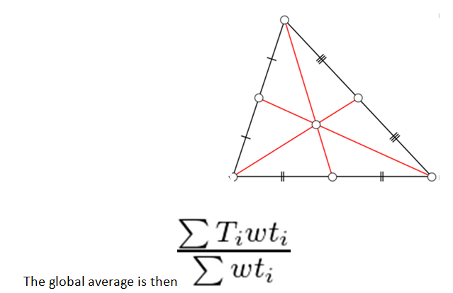
1. Each triangle contains one measurement at each vertex. We use Heron’s formula to calculate the area of the triangle.
2. Calculate the centroid position and assign this an anomaly equal to the average of all 3 vertex values. This centroid value is then used as the average anomaly for the whole triangular area.
3. Use a spatial weighting for each triangle in the integration equal to cos(lat)* area, where Lat is the latitude of the centroid of the triangle.

An example of such a triangulation grid is shown in Figure 1. 

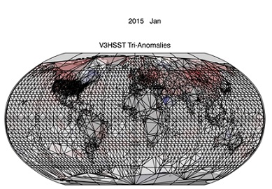Figure 1: A (lat,lon) triangulation mesh using all V3C station data and HadSST3 data

The second method extends triangulation to 3 dimensions. This has the advantage that it can now provide a full coverage of Polar Regions. This is an elegant method for spatial integration of irregular temperature data by using spherical triangulation over the earth’s surface. The method treats each measurement equally and covers the earth’s surface with a triangular mesh of station & SST nodes. Unlike linear 2D triangulation (described above) spherical triangulation also spans polar-regions because it uses a 3D model. Spherical triangulation returns the 3D Cartesian coordinates of each triangle vertex. The temperature of the triangular area is then set to the average of each vertex. The global average is the area weighted mean of all triangles. For the annual average we take the 12 monthly average of each global average. This is because the grid changes from one month to another. We investigate how to solve this in the third method (Figure 2). 

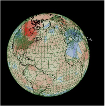Figure 2: Spherical triangulation of CRUTEM4 & HadSST3 (HadCRUT4.5) temperature data for January 2017. 

Spherical Triangulation essentially also solves the coverage bias problem for HadCRUT4, without the need for interpolation or use of external satellite data. Figure 3 shows a comparison of the Spherical Triangulation data to the Cowtan & Way data [3]. The agreement between the two is remarkable. This means that HadCRUT4 can already describe full global coverage, if it is treated in 3 dimensions instead of 2. 

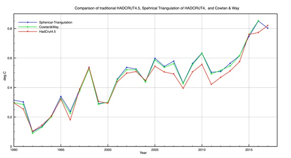Figure 3: Excellent agreement between Spherical Triangulation method andCowtan and Way. 2017 is incomplete and can be ignored.

The last method addresses the problem of defining unbiased fixed spherical grids in 3D. All the major temperature series use latitude, longitude gridding to average spatial temperatures. Problems arise near the poles, because bin sizes reduce as cos(lat), and the pole itself is a singularity. Spherical triangulation of monthly global temperatures is the most direct way to present temperature data, but it has one drawback. You cannot make annual or decadal averages directly on the triangular mesh, because it is forever changing from one month to another. You can only average monthly global averages together. To make such local averages you really need a fixed grid. So does that mean that we have to give up and return to 2D fixed lat,lon grids such as those used by CRU, Berkeley, NOAA or NASA? The answer is no because there is a neat method of defining fixed 3D grids that maintain spherical symmetry. This is based on subdividing an Icosahedron [7]. 

We start with a 20-sided icosahedron, which is a 3-D object all of whose sides are equilateral triangles. We then divide each triangle into 4 equal triangles by connecting each midpoint edge. These points are then extended outwards from the centre to lie on the surface of a unit sphere. The process is repeated n-times to form a symmetric spherical mesh as shown in Figure 4. It can be shown that such a grid formed from an icosahedron is the most accurate representation of a sphere (ref). 

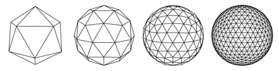Figure 4: Subdividing an Icosahedron to form a spherical grid. 

A level-4 icosahedron with 2562 triangles provides the best match to the actual distribution of HadCRUT4 global temperature data. An example of such a mesh, centered on the North Pole, is shown in figure 5. 

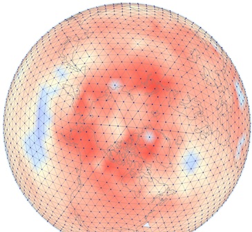Figure 5: Annual average (GHCN V3 & HadSST3) temperature anomalies for 2016. Note the equal area triangles covering the Arctic. 

The global anomaly is calculated by binning the data onto the grid in exactly the same way as is done for the 5x5 degree grid. A station lies within a given triangle if it is encircled exactly once. This is called the winding number. All stations within a given triangle and within a given time interval are then averaged. Such averages can be done monthly, annually or for each decade on the fixed grid. The global average is simply the numerical average over all bins, without any need for area weighting because they are all of the same area. Such grids allow annual and decadal averaging of temperature anomalies. Table 1 shows six successive decadal temperature averages calculated in this way using GHCNV3 and HadSST3, centered on Africa, while Table 2 shows the same decadal trends centered on the Arctic. 

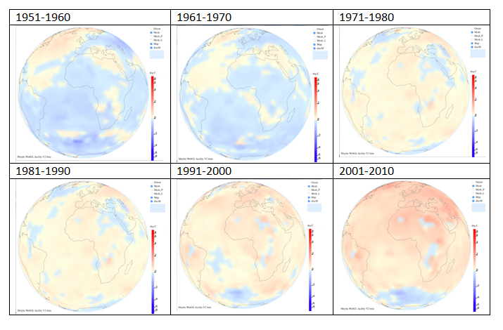                      Table 1: 10 year averages of temperature anomalies for GHCNV3+ HadSST3 on an isocahedral grid normalized to a 1961-1990 baseline. 

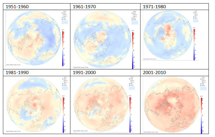Table 2: Decadal averages for Arctic regions. 

The results show a clear decadal warming trend after 1980 especially in the Arctic. Spatial results can be viewed in 3D e.g. http://clivebest.com/webgl/earth2016.html

CRUTEM4 station data and HadSST3 SST data have been processed using the three methods described above. These global averages have then been compared to HadCRUT4.5 data. Of the 7830 station data some 6857 have sufficient information to calculate anomalies and position them. A very small random perturbation has been added to the position of each SST data in order to triangulate them. This is because otherwise they would lie on exactly parallel latitude lines and the triangulation algorithm fails. Example triangulations are shown in figures 1 and 2.

A comparison of the annual values calculated by all 3 methods to the quoted HadCRUT4.5 values is shown in Figure 6. 

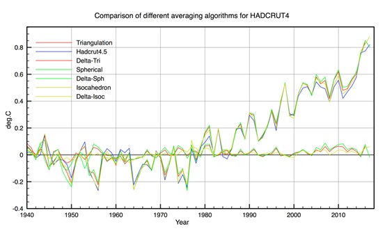Figure 6: HadCRUT4.5 Triangulation is Method1, Spherical is method 2 and Isocahedron is method 3. Deltas are the difference method-H4 

If instead of CRUTEM4 we use the NOAA GHCN V3C station data we get almost the same result. There are 300 more stations in V3C and although there is a large overlap, the homogenisation procedures are different. Figure 7 shows the comparison between the two plotted on the 1961-1990 baseline.

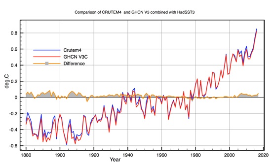 Figure 7: Comparison between GHCN V3C based annual averages and CRUTEM4 based annual avergaes. Both station samples are combined with HadSST3. 

In general the agreement between all three averaging methods is good. However there is a systematic difference after ~2000 between HadCRUT4.5 binning and the triangulation methods. This is due to the different processing procedures in Polar Regions. The spherical triangulation gives slightly higher net annual values than HadCRUT4.5 (up to 0.05C) after 2000. The monthly comparison is shown in Figure 8, excluding the icosahedral binning. The agreement is good but the same systematic effects are observed for the same reasons. The most interesting result is that Spherical Triangulation reproduces almost exactly the Cowtan and Way result. This shows that triangulation alone resolves any HadCRUT4 coverage biases in an internally consistent manner, without the need to use interpolation or bin averaging. 

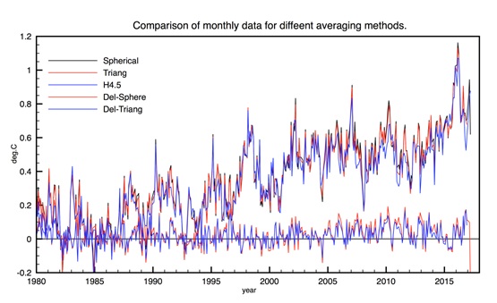Figure 8: Compare monthly anomalies. Black is Spherical triangulation, Red is lat. Lon triangulation and blue is HadCRUT4.5. Deltas show the same effect as the annual data. 

Another advantage of triangulation is that land ocean borders are respected in a consistent way. There is always a problem when averaging across a grid cell containing both land and ocean data. Ideally the average should be weighted by the fraction of land/ocean within the cell. This problem is avoided in triangulation because all measurements contribute equally irrespective of location.

We propose that for monthly averages the spherical triangulation method is the most accurate, because it does the best job of covering the poles. This conclusion is supported by the observation that it reproduces Cowatn & Way’s result, without the need for satellite data or kriging. The drawback of triangulation is that the grid is forever changing with time making spatial averaging difficult. For this reason icosahedral grids are proposed as optimum for annual or decadal averaging, although differences are small compared to latitude, longitude gridding. The traditional HadCRUT4.5 5x5 degree lat,lon binning is the most direct method, but it does slightly underestimate recent trends, which are concentrated in the Arctic. This is also partly because (lat,lon) cells can never span the poles.

All relevant software can be found at http://clivebest.com/data/t-study

Useful discussion and advice from Dr. Nick Stokes https://moyhu.blogspot.co.uk/

REFERENCES

- Robert Rohde, Richard Muller, Robert Jacobsen, et al. (2013) Berkeley Earth Temperature Averaging Process. Geoinfor Geostat 1:2.
- Osborn T, Jones P (2014) The CRUTEM4 land-surface air temperature data set: construction, previous versions and dissemination via Google Earth. Earth System Science Data 6: 61-68.
- Cowtan K , Way RG (2014) Coverage bias in the HadCRUT4 temperature series and its impact on recent temperature trends. Q J R Meteorol Soc 140: 1935-1944.
- Jones PD, Lister DH, Osborn TJ (2012). Hemispheric and large-scale land surface air temperature variations: an extensive revision and an update to 2010. Journal of Geophysical Research 117.
- Kennedy JJ, Rayner NA, Smith RO, et al. (2011) Reassessing biases and other uncertainties in sea-surface temperature observations since 1850 part 1: measurement and sampling errors. Part 1&2. J Geophys Res 116.
- Lawrimore JH, Menne MJ, Gleason BE, et al. (2011) An overview of the Global Historical Climatology Network monthly mean temperature data set, version 3. J Geophys Res 116.
- Wang N, Lee JL (2011) GEOMETRIC PROPERTIES OF THE ICOSAHEDRAL-HEXAGONAL GRID ON THE TWO-SPHERE. SIAM J SCI COMPUT 33: 2536-2559.
Citation: Best C (2020) Calculating Global Temperature Anomalies using Three New Methods. J Atmos Earth Sci 4: 023.
Copyright: © 2020 Clive Best, et al. This is an open-access article distributed under the terms of the Creative Commons Attribution License, which permits unrestricted use, distribution, and reproduction in any medium, provided the original author and source are credited.