Determination of Shale Microstructure from Laboratory Data on Permeability
*Corresponding Author(s):
Evgeni ChesnokovDepartment Of Earth And Ocean Sciences, University Of Houston, Houston, Texas, United States
Tel:+1 7137432579,
Email:emchesno@central.uh.edu
Abstract
The permeability of three shale samples is measured in laboratory at the conditions similar to in situ(confining pressure is 41.4 MPa and pore pressure is 20.7MPa). The effective medium theory is applied to invert parameters of shale microstructure from these measurements. Shale is modeled as a patched medium consisting of two types of patches related to (1) mineral matrix (2) pores and cracks. A double-porosity model is used to describe the pore/crack geometry of shale, which takes into account a degree of pore/crack connectivity. The inverted parameters of shale microstructure are used to predict the elastic wave velocities and thermal conductivity at in situ conditions in different directions relative to the bedding plane. The predicted values of velocities are in good correspondence with the velocities provided by sonic logs and laboratory data. The inverted permeability of “mineral matrix” and “fluid” patches can be used for theoretical prediction of the permeability tensor for shale having similar mineral composition and microstructure at the scale of laboratory measurements.
Keywords
Mineral matrix; Pores and cracks; Determination of Shale Microstructure
INTRODUCTION
At the scale of laboratory measurements (2 - 5 cm), the permeability of samples from Barnett Shale a gas shale formation (>60% carbonate,>20% Quartz and <20% Clay), located in the Bend Arch-Fort Worth Basin, Texas USA) measured in one direction on differently oriented samples give a possibility to reconstruct the permeability tensor. In this paper, we show such a reconstruction. However, these measurements require a complicated apparatus, special techniques depending on the rock type, and are rather time consuming. Another problem is to predict the permeability at another scale, for example, at the seismic scale. These facts lead to necessity of using theoretical methods to predict the permeability of anisotropic rocks.
Different theoretical approaches exist for estimating the hydraulic permeability of rocks at different scales. At the pore (or core) scale (microscale), the most popular are the empirical approaches, which relate the permeability with porosity and grain or pore size [11]. At this scale, using the Poiseuille’s and Darcy’s laws, Gueguen and Palciauskas [12] derived simple formulas for calculating the permeability of isotropic porous medium containing uniform distribution of capillaries having not greatly varying radii and lengths. They also derived similar formulas for cracks of known and not greatly varying aperture and diameter. This approach linearly relates the permeability and porosity both for capillaries and cracks. Another approach presented by Gueguen and Palciauskas [12] is based on the notion of hydraulic radius that is the ratio of pore volume to pore surface. This approach allows one to derive formulas relating the permeability and porosity for different pore/crack shape (tubes or cracks) taking into account the pore/crack density in terms of the percolation factor. In the case of capillaries, the permeability is the function of the squared porosity. For cracks, the permeability depends on the cube of porosity. The well-known Carman-Kozeny equation also follows from this approach. The formulas of this approach are semi-empirical since they contain a parameter to be fitted from the experimental data. The approaches for permeability determination at the mesoscale (when the size of a heterogeneity is much greater than the pore scale) are the topological theory, percolation theory, renormalization approach, homogenization approach, and geostatistical approach [13-20]. The approaches based on Effective Medium Theory (EMT) were used both at the core scale and at the mesoscale [21-25]. To date, this question: “Is the EMT suitable for the permeability calculation at this scale or not?”, is really debatable (a discussion at 13IWSA meeting). As follows from the empirical formulas, the permeability is controlled by size of grains, and the EMT does not incorporate these parameters. Thus, from this point of view, the EMT seems to be inapplicable to the permeability determination at the core scale. According to Vogel [13], who considered the permeability determination at different scales using the topological methods, the permeability is controlled by different parameters at different scales. Thus, Vogel [13] showed that the principal parameters controlling the permeability at the pore-scale level are the pore/crack connectivity and distribution of the pore volume over pore diameter. At the larger scale level, where a medium containing a set of pore and crack could be considered as macroscopically homogeneous (i.e., effective), the permeability is mainly controlled by statistical parameters of the hydraulic conductivity (mean and variance) and two-point correlation function of the hydraulic conductivity. Vogel [13] wrote that at this scale level, the pore-size effects are smeared by the statistical characteristics of their conductivity. The EMT does operate with the statistical characteristic, and from this point of view, the EMT is applicable at scales greater than the pore-scale level. The EMT was applied to determination of permeability at the mesoscale by Neuweiler and Vogel [23,25]. They employed the classical self-consistent scheme. More advanced approach of EMT to calculate the hydraulic permeability at the mesoscale, the T-matrix method of the quantum scattering theory, was applied by Jakobsen [24]. The T-matrix method allows one to take into account interactions between all pairs of inclusions (two-point approximation). This makes it possible to incorporate in the solution different spatial statistics (in the form of ellipsoids) for different types of inclusions. Note that the paper of Jakobsen [24] also contains a lot of references to recent works on permeability estimation in heterogeneous media.
Commonly, when applying EMT to calculate the effective permeability of a porous cracked medium at the mesoscale, the real medium is replaced by a patched medium with patches having different values of permeability. Pozdniakov and Tsang [23] and Jakobsen [24] considered the permeability of a sand-shale mixture taking the hydraulic conductivity 1 m/d for sand patches and 1e-4 m/d for shale patches. Neuweiler and Vogel [25] treated a porous-cracked medium like a material consisting of even five patches with different hydraulic conductivities. In this approach the size of patch is much greater than the pore/crack size, and EMT is applicable as follows from the topological models.
When applying EMT at the core scale for calculating the effective elastic properties and thermal or electrical conductivity, the medium is assumed to consist of two components: mineral material and voids. If we formally apply EMT to calculate its effective permeability from the properties of these components, we meet more difficulties as compared to the case when the permeability is calculated at the mesoscale or to the case when other effective properties (mentioned above) are calculated. Thus, a question about the permeability of solid matrix and fluid arises. Since the permeability is a characteristic of the pore/space geometry, the permeability of fluid through itself should be extremely large, and the permeability of mineral matrix (without pores and cracks) should be zero. However the contact of mineral grains is imperfect and, thus, the mineral matrix should not have zero permeability. Besides, according to empirical theories, the rock’s permeability at the core scale depends on the pore size. This means that if we formally apply the effective medium theory to two rock samples of the same porosity, pore/crack shape, fluid filling the pore space, and mineral composition but having different pore/crack size, we obtain the same results, which is not correct. Xu and White [21] proposed an estimate for the void’s permeability when applying the effective medium theory at the core scale. They use the value equal to
Note that a good review of many methods and approaches for calculating the equivalent permeability of a heterogeneous porous medium can be also found in Renard P and de Marsily G [27] .
Review of the some recently published papers related to our goals can be found in Kefey Lu, et.al.,[28], Aslan Gassiyev et.al [29] and Xianfu Huang , Ya-Pu Zhao [30]. In the last paper authors measured connectivity parameters and distinguish between isolated and connected porosity which is extremely important for permeability estimations.
PERMEABILITY CALCULATION WITH HELP OF EFFECTIVE MEDIUM THEORY
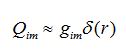
where r is the vector in 3D space, q(r) is the coordinate-dependent vector of fluid flux (discharge per unit area, with units of length per time, m/s), k(r) is the coordinate-dependent permeability tensor (of the 2nd rank), µ is the dynamic viscosity of fluid, and is the local pressure gradient. If the flow is steady state and there is no sources and sinks,
The Darcy law can be written in another form. If we introduce the hydraulic conductivity K by the formula (where ρ is the fluid density, and g is the gravity acceleration)
We can rewrite (1) as follows;
where
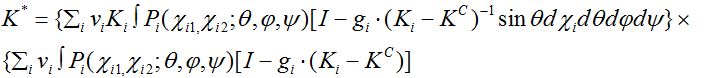
In formula (5) angular brackets mean averaging over the representative volume. A formal derivation of the effective hydraulic conductivity tensor using the generalized singular approximation method of the effective medium theory is given in Appendix. The formula for calculating the effective hydraulic conductivity has the form (see Appendix)
where tensor I is the fourth-rank unit tensor; tensor g depends on the inclusion’s shape and properties of the comparison body (see Appendix). Formula (6) includes the volume averaging. If the medium is statistically homogeneous, the volume averaging can be replaced by the statistical averaging (the ergodicity applies). We assume that all of the heterogeneities have the shape of general ellipsoid. The heterogeneities are assumed to be mineral grains and voids. If the heterogeneities differ in their physical properties, shape, and orientation in space, from formula (6) we have
 (7)
(7)We call the coefficient f in linear combination (8) friability. This empirical parameter can be treated as reflecting the degree of connectivity of Material 1. If the hydraulic conductivity of the matrix and Material 1 differ significantly, the HS bounds can be rather wide. Figure 1 shows the HS bounds calculated for a two-phase material with spherical inclusions. The hydraulic conductivity for the matrix and inclusions are taken as 1 and 10-4 m/day. This corresponds to the hydraulic conductivity of sand and shale [23]. Shale occupies 15% of the total volume. The effective hydraulic conductivity is also calculated for different values of friability entering expression (8). A strong non-linearity in dependence of effective hydraulic conductivity on friability is observed.In what follows we apply the generalized singular approximation method for calculating the permeability at the core scale. In so doing, we model a porous/crack rock by a patched medium consisting of patches related to mineral grains and Material 1. Material 1 replacing the pores and cracks has a finite (but rather high) scalar permeability.
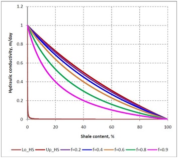 Figure 1: Effective hydraulic conductivity of sand-shale mixture versus shale content. “Lo_HS” and “Up_HS” are, respectively, the lower and upper Hashin-Shtrikman bounds, f is the friability (see formula (8)).
INVERSION OF THE MICROSTRUCTURE PARAMETERS OF SHALE SAMPLES
Laboratory measurements of shale permeability
The confining and pore pressure were 41.4 and 20.7MPa, respectively. According to our thought most of the cracks in gas shale studied are similar to tension racks. Thus, Walsh [35] approach (Pe = Pc-0.56 Pp) is used to calculate the effective pressure. Meanwhile, this approach gives the best fitting with the cubic κ-α law (where α is the stress) for the pressure range used in the current study. This effective pressure corresponds to the initial effective pressure in field, during water injection (hydro fracturing) of the gas shale formation from which these samples were taken. The liquid permeability values obtained for Sample 1 are 5, 12 and 21nano Darcy in the direction normal to bedding, 45° to bedding, and parallel to bedding, respectively. The respective values for Sample 2 are 22, 38 and 71nano Darcy for these directions, respectively. While these values for Sample 3 were 4, 8 and 15 nano Darcy. The average mineral composition of the samples studied are (in mass %): quartz 40%, carbonate (calcite and dolomite) 25%, total clay (illite, mixed layer and kaolinite) 27%, other minerals (pyrite, apatite and plagioclase) 8%. The measured porosity of the samples 1-3 are 5.9, 6.7 and 7.3%; the density is, respectively, 2.68, 2.61 and 2.64 g/cm3. The difference in permeability measured in different directions is attributed to the effect of horizontal cracks which are favorable for the fluid flow in the bedding plane and slower the fluid flow normal to bedding (Figure 2).
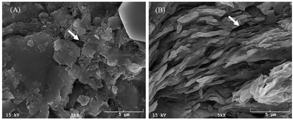 Figure 2: Scanning electronic microscope photographs show thermo-mature gas shale microstructure.
 (B) Parallel to the bedding view shows the well developed preferred orientation of the particles (alignment of platy minerals) and pores(white arrow).
The permeability measurements allow us to reconstruct the permeability tensors for these samples. Since the bedding plane is the symmetry plane, the permeability in this plane is independent of the azimuth and the components of the permeability tensor κ11 κ11 and κ22 are equal to one another. The permeability measured normal to bedding gives the value κ33 of the tensor. If the diagonal components of the permeability tensor are known, the permeability for any direction specified by the direction cosines n1, n2, n3 is calculated by the formula [36]:
Since for each of three samples we measured permeability at the angles 0, 45, and 90 degrees relative to the vertical axis of the samples (which is associated with the symmetry axis), we can check if the permeability is really related to the VTI symmetry. In order to do this, we find the values k11 and k33which simultaneously produce the best fit to permeability measured in the three directions (0, 45, and 90 degrees relative to the vertical axis). To find the values, we apply the least mean square method. The shale’s permeability changes only in the normal-to-bedding planes. The dependences of permeability on the polar angle are same for all normal-to-bedding planes. Figure 3 presents the permeability calculated by formula (10) with the values k11 and k33 producing the best fit to the experimental data. The maximum difference is seen for 45 degrees and varies from 6 to 15%. The difference in the experimental and theoretical permeability for 0 and 90 degrees is less than 5%. We should take into account these errors if we use VTI symmetry to characterize the permeability of the samples.
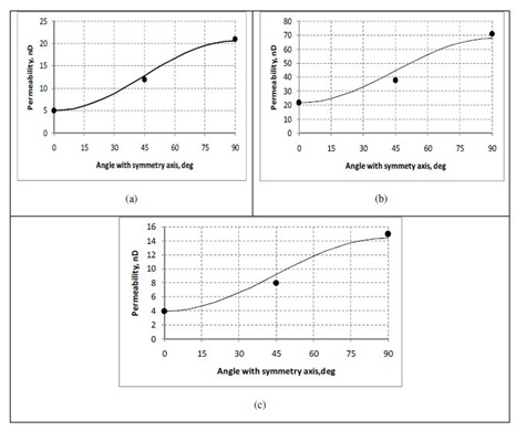 Figure 3: The permeability distribution in the vertical plane calculated by formula (10) with the values κ11 and κ33 producing the best fit to the experimental data (solid curves). The experimental values are shown by circles. (a) Samples 1, (b) samples 2, and (c) samples 3.
INVERSION OF SHALE’S MICROSTRUCTURE PARAMETERS
We assume that unknown parameters of shale’s microstructure entering formula (7) are as follows: friability, permeability of patches of solid material and “fluid” inclusions, crack porosity, aspect ratios of ellipsoids characterizing the patches of solid material, pore-related patches, and patches related to thin horizontal cracks. These parameters are found by minimization of the functional;
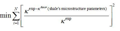
|
Sample |
“Matrix” permeability, nD |
“Fluid” penne ability, nD |
Friability |
Crack- patch aspect ratio |
Crack porosity, % |
Grain- patch aspect ratio |
Pore- patch aspect ratio |
Pore porosity, % |
|
|
Sample 1 |
9.4e-19±1.1e-19 |
498±34 |
0.78±0.009 |
0.02±0.001 |
0.31±0.02 |
0.17 ±0.04 |
0.85 ±0.02 |
4.7±0.07 |
|
|
Sample 2 |
1.3e-18±1.4e-19 |
1359±76 |
0.82±0.01 |
0.02 ±0.002 |
0.51±0.04 |
0.24 ±0.04 |
0.66 ±0.03 |
5.5±0.12 |
|
|
Sample 3 |
6.2e-19±1.0e-19 |
225±14 |
0.81 ±0.01 |
0.009±0.001 |
0.37 ±0.05 |
0.20 ±0.05 |
0.69 ±0.04 |
7.2 ±0.09 |
|
Table 1: The parameters of microstructure of shale samples inverted from the permeability measurements.
As seen, the “matrix” permeability is of the order 10-19-10-18 nano Darcy, and the “fluid” permeability range is 10-3-10-4 nano Darcy. The friability changes from 0.78 to 0.82. The aspect ratio of patches related to cracks is 0.01 - 0.02, and that for pores is 0.7 - 0.9. Grain patch aspect ratio varies from 0.17 to 0.2. This rather low aspect ratio of mineral-grain patches is explained by the fact that in our model we use a unified characteristic for silt-size grains that are isometric and clay platelets that are very thin. The crack porosity varies from 0.3 to 0.5%.
Note that the effective stiffness tensor and such tensor of thermal, electrical conductivity, and permittivity can be calculated from a formula similar to (6) [22]. However, for the elastic properties the tensor g is of the fourth rank and has the form,
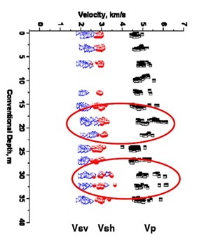 Figure 4: Measurements of Vp and Vs velocities along the well in the bedding plane of the Barnett Shale collection. These results show that all the samples are anisotropic. The average shear wave splitting is 30% [41].
|
Mineral |
Reference for corresponding stiffness tensor |
Vp, km/s |
Vs, km/s |
Density, g/cm3 |
|
|
Quartz |
McSkimin et al. [42] |
6.02 |
4.06 |
2.65 |
|
|
Calcite |
Peselnik and Robie [43] |
6.54 |
3.35 |
2.71 |
|
|
Dolomite |
Ahrens [44] |
6.4 |
3.46 |
2.86 |
|
|
Albite |
Belikov et al. [45] |
6.01 |
3.29 |
2.62 |
|
|
Pyrite |
Ahrens [44] |
7.86 |
5 |
5.02 |
|
Mineral |
Reference for corresponding stiffness tensor |
Vp, km/s |
Vs, km/s |
Density, g/cm3 |
|
|
Quartz |
McSkimin et al. [42] |
6.02 |
4.06 |
2.65 |
|
|
Calcite |
Peselnik and Robie [43] |
6.54 |
3.35 |
2.71 |
|
|
Dolomite |
Ahrens [44] |
6.4 |
3.46 |
2.86 |
|
|
Albite |
Belikov et al. [45] |
6.01 |
3.29 |
2.62 |
|
|
Pyrite |
Ahrens [44] |
7.86 |
5 |
5.02 |
The found parameters of shale microstructure are also used for a prediction of thermal conductivity for in situ conditions. Note that the thermal conductivity is a parameter which is not measured in wells like elastic wave velocities or resistivity. Therefore, such a prediction is of practical interest. Table 4 lists the thermal conductivity of minerals used for the prediction. The thermal conductivity of minerals and fluids is more sensitive to temperature compared to elastic properties. The thermal conductivity of fluids is also affected by pressure. This fact forces us to use the thermal conductivity of constituents at the respective PT conditions (effective pressure is 30 MPa and temperature is around 70 C°). The thermal conductivity for pyrite is taken for the normal conditions, since data at elevated PT conditions are unavailable for this mineral. We take into account the anisotropy of thermal conductivity of illite which is structurally similar to muscovite. We use Horai [46] data for the thermal conductivity of muscovite along the optical axis a and assume that the value along the axis b is the same. The thermal conductivity of illite along the optical axis c is calculated from the ratio of thermal conductivities of muscovite along the axis a and c given by Clark [47]. We also assume that the thermal conductivity of illite changes insignificantly with temperature like for clays presented in Material Properties Database [48]). When calculating the effective thermal conductivity we use the two-step model described above. The thermal conductivity of water and methane are taken equal to 0.68 and 0.0714 W/(m•K), respectively [49]. The theoretical prediction of effective thermal conductivity distribution in the vertical plane is shown in figure 5. The resulting in situ thermal conductivity is highly anisotropic. The thermal conductivity of shale samples in the bedding plane is 4.0 - 4.6 W/(m•K), whereas the value normal to bedding is around 1.8 W/(m•K). The ratio of thermal conductivity in the bedding plane to that normal to bedding is as high as 2.5. If we neglect anisotropy of illite and take the average value for thermal conductivity of isotropic illite equal 1.68 W/(m•K), the ratio decreases almost twice, down to 1.3. In this case, the thermal conductivity in the bedding and normal to bedding is around 4.2 and 3.3 W/(m•K).
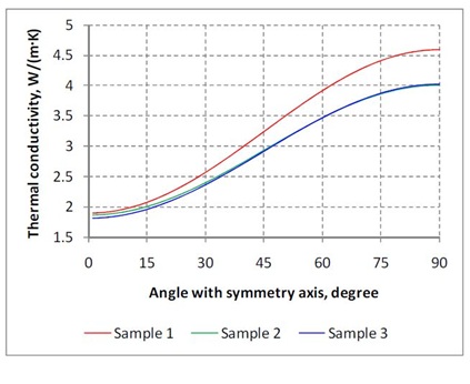 Figure 5: Theoretical prediction of the thermal conductivity distribution in the vertical plane.
|
Mineral |
Reference for corresponding stiffness tensor |
Vp, km/s |
Vs, km/s |
Density, g/cm3 |
|
|
Quartz |
McSkimin et al. [42] |
6.02 |
4.06 |
2.65 |
|
|
Calcite |
Peselnik and Robie [43] |
6.54 |
3.35 |
2.71 |
|
|
Dolomite |
Ahrens [44] |
6.4 |
3.46 |
2.86 |
|
|
Albite |
Belikov et al. [45] |
6.01 |
3.29 |
2.62 |
|
|
Pyrite |
Ahrens [44] |
7.86 |
5 |
5.02 |
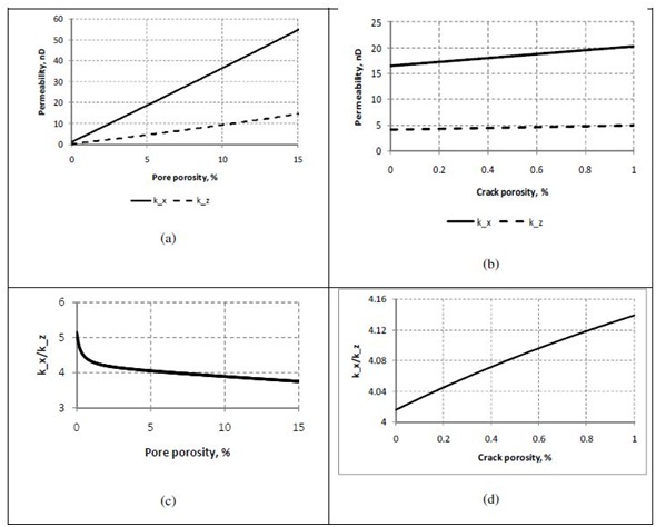 Figure 6: Theoretical analysis of permeability variation with (a) porosity of pores and (b) porosity of cracks; (c) and (d) are variation of ratio of permeability in the bedding plane to that normal to bedding plane with porosity of pores and cracks, respectively.
CONCLUSION
ACKNOWLEDGMENT
REFERENCES
- Kaarsberg EA (1959) Introductory studies of natural and artificial argillaceous aggregates by sound propagation and x-ray diffraction methods. Journal of Geology 67: 447-472.
- Vernik L (1993) Microcrack-induced versus intrinsic elastic anisotropy in mature HC-source shales. Geophysics 58: 1703-1706.
- Hornby BE, Schwartz LM, Hudson JA (1994) Anisotropic effective-medium modeling of the elastic properties of shales. Geophysics 59: 1570-1583.
- Johnston JE, Christensen NI (1995) Seismic anisotropy of shales. Journal of Geophysical Research 100: 599-6003.
- Vernik L, Liu X (1997) Velocity anisotropy in shales: A petrophysical study. Geophysics 62: 521-532.
- Lonardelli I, Wenk HR, Ren Y (2007) Preferred orientation and elastic anisotropy in shales. Geophysics72: 33-40.
- Wenk HR, Lonardelli I, Franz H, Nihei K, Nakagawa S (2007) Preferred orientation and elastic anisotropy of illite-rich shale. Geophysics 72: 69-72.
- Mohamed Y (2007) Physico-chemical behaviors of shale/fluid/solute interaction in geo-environmental and geo-engineering applications. University of Norman, Oklahoma, USA.
- Ohmyoung K, Kronenberg AK, Gangi AF, Johnson B, Herbert BE (2004) Permeability of illite-bearing shale: 2. Influence of fluid chemistry on flow and functionally connected pores. Journal of Geophysical Research
- Clennell MB, Dewhurst DN, Brown KM, Westbrook GK (1999) Permeability anisotropy of consolidated clays. Geological Society 158: 79-96.
- Odong J (2007) Evaluation of empirical formulae for determination of hydraulic conductivity based on grain-size analysis. Journal of American Science 3: 54-60.
- Gueguen Y, Palciauskas V (1994) Introduction to the Physics of Rocks. Princeton University Press, Princeton, New Jersey, USA.
- Vogel HJ (2002) Topological characterization of porous media. In: Mecke KR, Stoyan D (eds.). Morphology of Condensed Matter: Physics and Geometry of Spatially Complex Systems, Lecture Notes in Physics 600: 75-92.
- Adler PM, Mourzenko VV, Throvert JF, Bogdanov I (2005) Dynamics of Fluids and Transport in Fractured Rock. In: Faybishenko B, Witherspoon PA, Gale J (eds.). Study of single and multiphase flow in fractured porous media, using a percolation approach. Geophysical Monograph Series Washington, US A. Pg no: 33-41.
- Hilfer R (1992) Local-porosity theory for flow in porous media. Physical Review B 45: 7115-7121.
- King PR (1989) The use of renormalization for calculating effective permeability. Transport in Porous Media 4: 37-58.
- Aharony A, Hinrichsen EL, Hansen A, Feder J, Jøssang T, et al. (1991) Effect of pore pressure and confining pressure on fracture permeability. Physica A: Statistical Mechanics and its Applications 177: 260-266.
- Rohan E (2006) Homogenization approach to the multi-compartment model of perfusion. Proceedings in Applied Mathematics and Mechanics 6: 79-82.
- Kitanidis P, Vomvoris EG (1983) A geostatistical approach to the inverse problem in groundwater modeling (steady state) and one-dimensional simulations. Water Resources Research 19: 677-690.
- Kitanidis P (1996) On the geostatistical approach to the inverse problem. Advances in Water Resources 19: 333-342.
- Xu S, White RE (1996) Modeling transport properties of anisotropic shaly formations. Society of Exploration Geophysicists, SEG Annual Meeting, Oklahoma, USA. Pg no: 1063-1066.
- Bayuk IO, Chesnokov EM (1998) Correlation between elastic and transport properties of porous cracked anisotropic media. Journal of Physics and Chemistry of the Earth 23: 361-366.
- Pozdniakov S, Tsang CF (2004) A self-consistent approach for calculating the effective hydraulic conductivity of a binary, heterogeneous medium. Water Resources Research
- Jakobsen M (2007) Effective hydraulic properties of fractured reservoirs and composite porous media. Journal of Seismic Exploration 16: 199-224.
- Neuweiler I, Vogel HJ (2007) Upscaling for unsaturated flow for non-Gaussian heterogeneous porous media. Water Resources Research 43.
- Holt RM, Kolstø MI, (2017) How does water near clay mineral surfaces influence the rock physics of shales? Geophysical Prospecting 65: 1615-1629.
- Renard P, de Marsily G (1997) Calculating equivalent permeability: a review. Advances in Water Resources 20: 253-278.
- Kefei Lu, Metwally YM, Dyaur N, Chesnokov EM (2015) BARNETT Shale Velocity and Permeability Anisotropy Measurements. Quarterly Physics Review 2: 1-23.
- Gassiyev A, Huang F, Chesnokov EM(2016) Using the pair-correlation function as a tool to identify the location for shale gas/oil reservoir based on well-log data. Geophysics 81: 91-109.
- Huang X, Zhao YP (2017) Characterization of pore structure, gas adsorption, and spontaneous imbibition in shale gas reservoirs. Journal of Petroleum Science and Engineering 159: 197-204.
- Sasaki T, Watanabe K, Lin W, Hosoya S (2003) A study on hydraulic conductivity for Neogene sedimentary rocks under low hydraulic gradient condition. Shigen-to-Sozai 119: 587-592.
- Willis J (1977) Bounds and self-consistent estimates for the overall properties of anisotropic composites. Journal of Mechanics and Physics of Solids 25: 185-202.
- Shermergor TD (1977) Theory of Elasticity of Microinhomogeneous Media. Moscow ISBN 20304-135/053(02)-77 150-77 (in Russian).
- Hashin Z, Shtrikman S (1962) A Variational Approach to the Theory of the Effective Magnetic Permeability of Multiphase Materials. Journal of Applied Physics 33: 3125-3131.
- Walsh JB (1981) Effect of pore pressure and confining pressure on fracture permeability, International Journal of Rock Mechanics and Mining Science & Geomechanics Abstracts 18: 429-435.
- Heinbockel JH (2001) Introduction to Tensor Calculus and Continuum Mechanics. Trafford Publishing, Bloomington, USA.
- Bayuk IO, Ammerman M, Chesnokov EM (2007) Elastic moduli of anisotropic clay. Geophysics 72: 107-117.
- Bagrintseva KI (1982) Cracks in sedimentary rocks. Nedra, Moscow (in Russian).
- Bayuk I, Ammerman M, Chesnokov E (2008) Upscaling of elastic properties of anisotropic sedimentary rocks. Geophysical Journal International 172: 842-860.
- Tiwary DK, Bayuk I, Vikhorev A, Chesnokov E (2009) Comparison of seismic upscaling methods: From sonic to seismic. Geophysics 74: 3-14.
- Dyaur N, Kullmann G, Ortiz A, Pena V, Chesnokov E (2008) Velocity Anisotropy and X-ray imaging of Barnett shale. Society of Exploration Geophysicists, SEG Annual Meeting. Oklahoma, USA. Pg no: 554-558.
- McSkimin HJ, Andreatch P, Thurston RN (1965) Elastic moduli of quartz versus hydrostatic pressure at 25° C and -195.8° C. Journal of Applied Physics 36: 1624-1632.
- Peselnick L, Robie RA (1962) Elastic constants of calcite. Journal of Applied Physics 33: 2889.
- Ahrens TJ (1995) Rock Physics & Phase Relations: A Handbook of Physical Constants. American Geophysical Union, Washington,
- Belikov BP, Aleksandrov KS, Ryzhova TV (1970) Elastic Constants of Rock- Forming Minerals. Nauka (in Russian).
- Horai K (1971) Thermal conductivity of rock-forming minerals. Journal of Geophysical Research 76: 1278-1308.
- Clark SM (1966) Handbook Physical Constants of Rocks. The Geological Society of America,Yale University, New Haven, Connecticut, USA.
- JAHM (2017) Temperature Dependent Material Properties Database. Material Properties Database (MPDB), JAHM Software Inc.
- Vargaftik NB, Vinogradov YK, Yargin VS (1996) Handbook of physical properties of liquids and gases. Begell House, Connecticut, USA.
- Torquato S (2002) Random heterogeneous materials: microstructure and macroscopic properties. Springer Publishing, New York, USA.
- Elliot RJ, Krumhansl JA, Leath PL (1974) The theory and properties of randomly disordered crystals and related physical systems. Reviews of Modern Physics 46: 465-542.
- King PR (1987) The use of field theoretic methods for the study of flow in a heterogeneous porous medium. Journal of Physics A 20: 3935-3947.
APPENDIX
where is the derivative of a function with respect to coordinate a (a = 1, 2, 3).
Let us consider a homogeneous body (so-called comparison body) having the same shape as the heterogeneous body for which eq. (4) in section “Formal derivation of the effective permeability tensor” is written. We assume that the comparison body is subject to the same boundary conditions as the heterogeneous body. The Darcy law in the form (A2) for the homogeneous body takes as written as follows
Subtracting (A3) from (A2), we obtain
where
We determine the Green’s function G of operator LC as follows
where is the Dirac delta distribution. The solution to (A5) has the form
where the star operator means convolution.
According to eqs. (A6) and (A1), the i-th compone
nt of can be written as follows;

Where When performing integration by parts in equation (A7), it is taken into account that
Shermergor [33] demonstrated that for bodies of rather great size the surface integral can be neglected. If we consider a volume of rock large enough compared to the heterogeneity size, we can do this. In this case, we have,

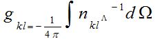
where Q is the integral operator. Equation (A8) is similar to the Lippmann-Schwinger equation of the quantum theory [51]. Similar derivation could be also found in King [52]. In generalized singular approximation method, the operator Q that is replaced by a constant tensor with the use of the formula [33],
Using such a replacement, we neglect the coordinate dependence of the second derivative of the Green function and obtain the solution in so-called one-point approximation. In this case, the gradient of the hydraulic head is homogeneous within each heterogeneity type.
Shermergor [33] derived formulas for tensor g in the case of elasticity. He used the Fourier transforms of the equation for the Green function similar to (A6) and assumed that heterogeneities have ellipsoidal shape. Applying the same way of the derivation, we have
Where
 and ai are the semi-axes of the ellipsoidal inclusions;
 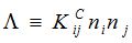 .
.Formula (A10) gives a possibility to consider general ellipsoids (with three different semi-axes) whereas the use of depolarization tensor for similar computations allows one to use only ellipsoids of revolution [23]. Note that Willis [32] derived a tensor analogous to (A10) for the case of effective thermal conductivity.
Replacing operator Q by tensor g in (13), we have (in the tensor form)
After some algebraic rearrangements, from eq. (A11), we can obtain a relation between the hydraulic head gradient at a point r in the heterogeneous body and the volumetric average of this gradient in the body:
where I is the unit tensor of the second rank. Applying to equation (A12) the definition of effective tensor of hydraulic conductivity (equation (5) of this paper), we obtain
Note that formula (A13) is suitable for any transport properties described by the equation having the form of (A2). For example, it can be applied for calculation of the effective thermal and electrical conductivity, and permittivity.
Citation: Chesnokov E, Bayuk I, Metwally Y (2017) Determination of Shale Microstructure from Laboratory Data on Permeability. J Atmos Earth Sci 1: 003.
Copyright: © 2018 Evgeni Chesnokov, et al. This is an open-access article distributed under the terms of the Creative Commons Attribution License, which permits unrestricted use, distribution, and reproduction in any medium, provided the original author and source are credited.