Global Surface Temperature Variability and Trends and Attribution to Carbon Emissions
*Corresponding Author(s):
Pietrafesa LJCenter For Marine And Wetland Studies, Department Of Marine, Earth And Atmospheric Sciences, North Carolina State University, Coastal Carolina University, South Carolina, North Carolina, United States
Tel:+1 7049107047,
Email:len_pietrafesa@ncsu.edu
Abstract
Keywords
Attribution of anthropogenic influence in climate change; Climate change; Climate warming; Fossil fuel burning; global surface atmospheric temperature anomalies; Global warming; Patterns of climate variability; Sea and ocean surface temperature anomalies
INTRODUCTION
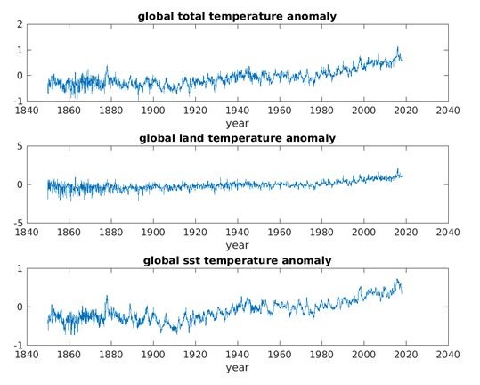
In the study reported on below, we will revisit the temperatures of the global surface of the earth (upper panel in figure 1), the atmosphere above land (middle panel in figure 1) and the surface of the global ocean (lower panel in figure 1) from 1850 through the first half of 2018. We will employ the well-known and documented surface-temperature-anomaly-data. While much attention has focused on the global surface atmospheric temperature record, as greenhouse gases have built up in the atmosphere, far less attention has been paid to the global ocean surface temperature record in-kind. We will investigate the variability of land and ocean surface temperatures and determine if we can shed new insights into what is revealed regarding the present state of the Earth’s climate system.
The climate system consists of non-linear and non-periodic processes, so we will utilize an empirical, mathematical, data adaptive technique to decompose the data. Our mathematical decomposition methodology produces internal, intrinsic modes of variability buried within the temperature time series that can be replicated with sine functions and thus can be considered quasi-stationary. “Nonlinear” (NL) is defined as a time series of systems governed by equations more complex than the linear form, ????=???? ????+????, where ‘a’ and ‘b’ are constants. We will account for the patterns revealed by the internal modes of variability, relate them to naturally occurring physical phenomena and then compute the overall trends which we find does not have a natural causal basis. Consequently, we will employ a statistical hypothesis test for determining whether one time series, such as fossil fuel burning, can be useful in forecasting another, specifically global surface temperatures and thus to predict climate warming, past, present and future; thus causality.
BACKGROUND AND METHODOLOGY
In discussing the trend of any time series, we first need to consider the definitions and the methodologies of computing a trend, as this is especially important for temperature time series. As such, no conventional simple averaging process can be utilized to reflect what information is buried in the multiple temperature time series. This underscores the importance of clearly defining what constitutes a trend. Granger [14], presented an insightful definition of a trend as “a trend in mean comprises all frequency components whose wavelength exceeds the length of the observed time series”. In the mathematical treatise of definitions of James and James [15], the definition of a trend is stated to be “the general drift, tendency or bent of a set of data”. Chatfield [16], defines “trend” as “a long-term change in the mean”. Thus, difficulties arise in determining what “long term” means. For example, a 50-year cycle would appear to be a trend in a 20-year data set; but it would be shown as a 50-year cycle when the length of the data was longer than 50 years. In speaking of a “Chatfield trend” we must take into account the number and span of observations available and then make a subjective assessment as to what constitutes “long term”. For NL, NS datasets, none of these definitions is mathematically applicable leading to employment of the definition based on the work developed in Wu et al. [17]. In that paper, the EMD decomposition included the non-oscillation “residue”, after the higher to lower frequency modes, the Intrinsic Mode Functions (IMFs), in the global surface temperature anomalies (the GSTA) were removed in the time varying decomposition. The authors then called that residue the trend.
Thus, given our discussion above, prior to the revelation of Wu et al. [17], there was not an applicable definition of what constituted the overall “trend” of any continuous time series of data, especially of a non-linear NL time series. As such, a well mathematically defined methodology of how to compute a trend of a time series had not existed in the literature. This work presented a logical definition of a trend as an intrinsically determined function within the temporal span of the data, in which there can be at most one extremum. Being intrinsic, the method to derive a trend was adaptive; that is, it suited the span of the data. Thus, the definition of a trend in this publication presumed that a time scale exists that is logically and mathematically related to the span of the data, and was in keeping with the definition suggested previously by Granger [14]. With this definition of a trend, we will employ the EEMD method [13], to decompose the time series of global ocean surface temperature and air temperature above land surface, from 1850 through July 2018, and identify all of their intrinsic modes and trends.
GLOBAL OCEAN AND LAND BASED ATMOSPHERIC TEMPERATURE ANOMALY TIME SERIES
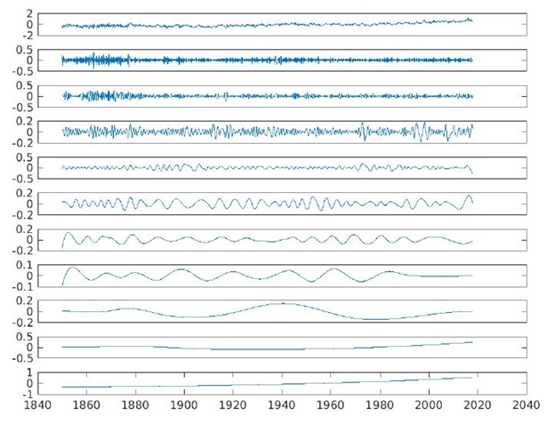
Figure 2 shows eleven IMF modes in the GSTA (also true of the GLSTA and GOSTA, so not shown) with the 11th being the overall trends of the land-based atmosphere, the ocean surface and the combination of the two. The IMF modes of the GOSTA and GLSTA are essentially the same for the ocean surface and for the atmosphere over land, save for differing amplitudes. The IMF modes have their respective physical basis. Mode 1 is several monthly variability. Mode 2 is seasonal variability. Mode 3 is the motion of the Earth on its axis of rotation. Mode 4 is the annual signal. Mode 5 is inter-annual variability. Mode 6 is the dominant signal of the El Nino Southern Oscillation (ENSO). Mode 7 is the quasi-Solar Cycle (10-12 years), centered about 11 years. Mode 8 reflects both the North Atlantic Oscillation (NAO) and of the 22-year Solar Cycle. Mode 9, 60-70 years is the Atlantic Meridional Overturning Circulation Belt (MOC), described by Cunningham et al., [19]. Mode 10, 105-110 years represents the global thermohaline circulation conveyor belt [20,21]. Mode 11 is the gravest mode or overall trend of the 167-year time series of total data (Table 1).
|
IMF |
1 |
2 |
3 |
4 |
5 |
6 |
7 |
8 |
9 |
10 |
11 |
|
GLSTA |
2 M |
3M |
6M |
1Y |
2-3Y |
5-7Y |
10-12 Y |
20-22Y |
60-70Y |
105-110Y |
167Y Trend |
We note in figure 2, that for the GSTA, the IMF modes 2, 3 and 10 have amplitudes of 0.4oC, modes 4 and 6 have amplitudes of 0.3°C, modes 5, 7 and 9 have amplitudes of 0.2°C and mode 8 amplitude of 1°C. Mode 11 ranges between +/- 0.5°C. Thus, all the IMF modes contribute to the total time series in temperature amplitudes in a nominally equitable manner across the range of 0.1 to 0.4°C. This finding suggests that the Planet’s internal, natural modes of variability contribute all contribute significantly to monthly averaged surface temperatures and thus cannot be ignored. Thus, periods of relative warming and or cooling occur naturally by the positive and negative disposition of the natural variability, all riding atop overall atmospheric and oceanic trends and presented in the table below.
In figure 3, the overall trends of the GOSTA, GLSTA and GSTA are presented relative to each other, from their anomaly starting points January 01, 1850 to their end values December 31, 2017.
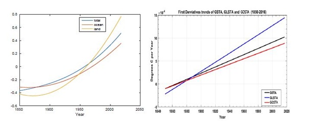
In figure 3 (left panel), the trend of the GLSTA shows a record length total rise of 1.22°C and the GOSTA displays a total rise of 0.67°C. The GSTA or combined ocean surface and land surface rises 0.88°C. The ocean surface temperature GOSTA has risen at a much slower rate than the atmosphere over land, the GLSTA. This is an excellent example of the power of the EEMD IMF decomposition. The full time series of the GOSTA displays an overall beginning to end of the series increase of 0.75°C, the GLSTA shows a rise of 2.91°C and the GSTA indicates an overall increase of 1.25°C. If connecting lines from start to end of the three time series had been drawn, the overall trends would have been greatly overestimated, demonstrating the failing of traditional methods of computing a trend, which are to create regression lines. Thus, the IPCC rates of rise of GSTA (IPCC, 2007) overestimated the actual rises in temperatures over land by 0.72°C and by a combined air-sea overestimate of 0.37°C. The IPCC straight-line, regression slope estimates were 0.05°C/decade over the full GSTA temperature record, 0.07°C/decade over the prior 100 years, 0.13°C/decade over the previous 50 years and 0.18°C/decade over the latter 25 years of the record. It is of note that the GSTA temperature time series is the same time series, from the identical source, <http://www.cru.uea.ac.uk/cru/info/> that we used in our analyses.
In figure 3 (right panel), we present the time rates of our trends (Figure 3, left panel). We find that the rates of warming from 1850 through 2017 are 7.13(10-2) °C/decade for the GLSTA, 4.27 (10-2) °C/decade for the GOSTA, and 5.29 (10-2) °C/decade for the combined GSTA. However, the 1st derivatives of the trend curves are all positive and curving upward indicating that the rate of warming is accelerating. More recently, from 1955 to the present the overall warming trend of the GSTA (Figure 3) has been about 8.83(10-2) °C/decade. Clearly, the rate of warming of air over land has globally been 167% greater than that of the surface of the global ocean. The temperature anomaly trends all range from negative values at the onset of each of the time series in 1850 to highly positive values at the end of 2017. Thus, employing straight regression lines is not the mathematically or physically plausible manner in which trends of non-linear time series can be estimated. Only an adaptive method such as EEMD [13] can do so, as explained above [22]. We also note from figure 3 that from 1850 to 1895 the air temperature trend over land actually decreased slightly, so there was a slight global cooling over land globally that persisted for about 45 years. Then in 1895, the global air temperature over land reached its prior value in 1850 and then continued to rise through 2017. The scenario was essentially flat for the global ocean with warming commencing about 1880. The combined atmosphere and ocean time series follows closely to that of the ocean and moved from slight cooling to warming about 1880. The air over land was relatively cooler than that of the surface of the ocean until about 1915 when the trend lines cross and air temperatures on land rose at a more rapid rate than did those of the ocean. The air over land and ocean surface trend curves have diverged significantly up through 2017.
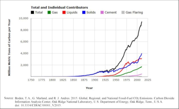
FOSSIL FUEL BURNING, CARBON EMISSIONS AND CO2
GRANGER CAUSALITY RELATING CARBON BURNING TO GLOBAL SURFACE TEMPERATURE ANOMALIES
First, we conducted a series of cross-correlations between surface temperature anomalies and fossil fuel burning. We started with the Earth’s surface temperatures (GLSTA, GOSTA and GSTA) leading the fossil fuel burning curve (CE). We found, by way of example, that the lagged value of GOSTA provides no statistically significant improvement in predicting the CE. Therefore, one cannot establish that global surface temperature changes (such as the GOSTA) “causes” the CE change outcome in the same manner as suggested above and discussed next below. For example, a fourth order autoregressive model, which fits the data starting in 1950 to {xt} using the previous year GOSTA {yt-1}, results in a p-value of only 0.65 of the significance of the coefficient for GOSTA. We would definitely not conclude that GOSTA is causing outcomes for CE. Now we move onto demonstrating the effect or lack thereof that CE has on the GOSTA and by association on the GLSTA and GSTA (both not shown).
We first consider establishing a causal relationship between the carbon burning time series ({xt}) and the ocean surface temperature time series GOSTA ({yt}) in the latter half of the 20th century. Here we model on the monthly scale by taking the average temperature anomaly for each year as y and the average monthly carbon emission created by taking the yearly value divided by 12. Our first model relates GOSTA to past values of GOSTA. Using Akiake’s Information Criterion [29] we select the order of the auto regression to be three, meaning that each year’s GOSTA is related to the values from the last 3 years. The model is fitted using Gaussian maximum likelihood [30]. We use the goodness of fit test [28] to verify that the AR model adequately models the autocorrelation in the GOSTA series; the p-value of 0.9464 indicates that we have found an adequately fitting stationary model for GOSTA model given in Equation (1):
????????=0.00925+0.7676????????-1-0.2575????????-2+0.4264????????-3+???????? (1)
The above model explains the dynamics of the observed series solely from past-observed values. We note that we could improve the predictive ability the above model by adding a linear trend component and would do so if our goal was to estimate the rate of change of temperature. However, to establish the (Granger) causal relationship we instead add the previous year CE value to the model. The resulting model is given by Equation (2):
????????=-0.054+0.6605????????-1-0.2772????????-2+ 0.3376????????-3+0.0007????????-1+???????? (2)
We can test for statistical significance of each fitted coefficient using the asymptotic normality of the Gaussian maximum likelihood estimators [30]. In particular, we conclude with a p-value of 0.00009 that the coefficient of xt-1 is non-zero. In other words, the predictive model for GOSTA is significantly statistically better if the previous year CE is included. Model (2) explains the changes in temperature through a combination of autocorrelation (AR) and the impact of CE. We have thus established causality in the granger sense. In this analysis, we selected the data beginning in 1950, since the warming trend in the latter half of the 20th century is well established (cf. figure 3). However, a similar analysis could be conducted starting at any point in the past. For example, the same analyses beginning each decade in the first half of the 20th, i.e. in years 1900, 1910, 1920, 1930, 1940 and 1950, resulted in p-values, 0.00005, 0.0002, 0.00002, 0.0002, 0.003, 0.009, for the coefficient of xt-1, respectively. In each case we conclude the model using the previous year CE is statistically better than the AR (3) model alone; the carbon emission series significantly improves predictions for GOSTA over the model based solely on past GOSTA values. Regardless of starting time, in the 20th century, one finds statistical evidence of a causal relationship between CE and GOSTA.
The coefficient for xt-1 in model (2) is as follows. For each additional one-million metric tons of Carbon Emissions (CE), we estimate an increase in Global Ocean Temperature (GOSTA) of 0.0007 °C. The average increase in carbon emissions per year for years 1950 through 2014 is about 130 metric tons per year. Our model estimates an increase of 0.007+ °C for each 10 metric ton increase in carbon emissions. The highly statistically significant coefficients of xt-1 for land based atmospheric temperatures and total global surface temperatures are 0.0117 and 0.0087, respectively.
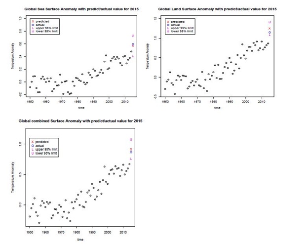
We next employ our fitted models to predict the global sea surface anomaly (GOSTA), the land atmosphere (GLSTA) and combined Global Surface Temperature Anomalies (GSTA) for 2015. Figure 5 shows the observed anomalies for years 1950 through 2014. The prognostic values are remarkably accurate. In the plots, we mark the predicted value from our fitted model, the upper and lower 95% prediction limits and the observed value for Year 2015. We find that the model, which uses both past values of the anomaly series and the previous year’s carbon emission, provides excellent predictions for the observed anomalies of the ocean surface, atmosphere on land and the combination therein for 2015. This provides further empirical evidence of Granger Causality relating previous year carbon emissions to sea surface, atmosphere on land and the combination temperatures on a global scale. We utilized the 2014 and 2015 data because 2014 is the last year for which we were able to obtain Fossil Fuel Burning data from the website provider at the time that this study was conducted.
The results presented above provide a pathway and portend to future increases in global surface temperatures given anticipated increases in fossil fuel burning, GOSTA, GLSTA and GSTA as a function of CE. GOSTA is increasing at the rate of 0.0007°C/ Million Metric Tons of CE. GLSTA is increasing at the rate of 0.00117°C/Million Metric Tons of CE. Thus, the GSTA is increasing at the rate of 0.00087°C/Million Metric Tons of CE. Presently we are on a trajectory to reach 104 Million Metric Tons/year of CE by years 2020 to 2022. While these numbers are less foreboding than the straight-line estimates of both the IPCC and NIPCC, they are nonetheless very noteworthy.
DISCUSSION AND CONCLUSION
Empirical relationships between billions of tons of fossil fuel burning and the overall trends of the global surface-temperature-anomaly-time series in both the global ocean, the air above land and the combined time series emerge from our reduction of the non-stationary, non-linear data. Mathematical relationships between fossil fuel burning and surface temperatures in the oceans and over land are presented. The statistical relationship curves reveal strongly that there is a one-year phase lag between global carbon loading via fossil fuel burning and planetary surface temperature rise, different from Ricke and Caldeira [31], who proposed that planetary temperatures changed about a decade after burning. In fact, robust relationships are presented between the GLSTA, GOSTA and GSTA, and their past time series and the CE time series. Via Granger Causality, these surface temperatures are predicted very accurately from fossil fuel burning a year earlier. Thus, the conclusion we reach is that we have proven that there is “attribution” between fossil fuel burning and climate warming [32-41].
In 2007, the IPCC was awarded a Nobel Prize for its visual-correlative-comparison of fossil fuel burning and temperature rise. However, a visual correlation does not prove “causality”. In 2003 CWJ Granger was awarded a Nobel Prize for his work in econometrics theory and applications. We invoked “Granger Causality” to attribute the overall trends in global surface warming to fossil fuel burning and carbon emissions (https://en.wikipedia.org/wiki/Clive_Granger).
The conclusion reached in this study of overall planetary temperature trends versus the time series of fossil fuel emissions is that if present fossil fuel burning is not curtailed there will be continued warming of the planet in the future. We find that while the global ocean has an enormous capacity to absorb and retain heat and thus act as a planetary heat reservoir, it is releasing stored heat in increasing amounts over time. Our findings are causally correlative in the sense of Granger Causality [23] and this study definitively links the overall trends in planetary surface temperature rise, to the overall upward trend in fossil fuel burning.
ACKNOWLEDGEMENT
REFERENCES
- Bernstein L, Bosch P, Canziani O, Chen Z, Christ R, et al. (2008) IPCC, 2007: Climate change 2007: Synthesis report. Geneva, Switzerland.
- Stocker TF, D Qin, GK Plattner, M Tignor, SK Allen, et al. (2013) Climate Change 2013: The Physical Science Basis. IPCC, Geneva, Switzerland. Pg no: 1535.
- Al?Ghussain L (2019) Global warming: Review on driving forces and mitigation. Environmental Progress & Sustainable Energy 38: 13-21.
- Allen MR, Frame DJ, Huntingford C, Jones CD, Lowe JA, et al. (2009) Warming caused by cumulative carbon emissions towards the trillionth tonne. Nature 458: 1163-1166.
- Ekwurzel B, Boneham J, Dalton MW, Heede R, Mera RJ, et al. (2017) The rise in global atmospheric CO2, surface temperature, and sea level from emissions traced to major carbon producers. Climatic Change 144: 579-590.
- Heede R (2014) Tracing anthropogenic carbon dioxide and methane emissions to fossil fuel and cement producers, 1854-2010. Climatic Change 122: 229-241.
- Millar RJ, Fuglestvedt JS, Friedlingstein P, Rogelj J, Grubb MJ, et al. (2017) Emission budgets and pathways consistent with limiting warming to 1.5 °C. Nature Geoscience 10: 741-747.
- Smith CJ, Forster PM, Allen M, Fuglestvedt J, Millar RJ, et al. (2019) Current fossil fuel infrastructure does not yet commit us to 1.5 °C Nature Communications 10: 1-10.
- Millar RJ, ZR Nicholls, P Friedlingstein, MR Allen (2016) A modified impulse-response representation of the global response to carbon dioxide emissions. Atmos chem phys discuss. Pg no: 1-20.
- Huang NE, Shen Z, Long SR, Wu MC, Shih EH, et al. (1998) The empirical mode decomposition and the Hilbert spectrum for nonlinear and non-stationary time series analysis. Proc Roy SocLond 454: 903-993.
- Gabor D (1946) Theory of communication. J IEE 93: 429-457.
- Van der Pol B (1946) The fundamental principles of frequency modulation. IEE 93: 153-158.
- Wu Z, NE Huang (2009) Ensemble Empirical Mode Decomposition: A noise-assisted data analysis method. Advances in Adaptive Data Analysis 1: 1-41.
- Granger CWJ (1966) The Typical Spectral Shape of an Economic Variable. Econometrica 34: 150-161.
- James and James (1976) The Mathematical Dictionary. (4th Edn). D. Van Nostrand Com. Publisher.
- Chatfield C (2003) The analysis of time series, An introduction (6th edn). Chapman & Hall/CRC, Florida, USA.
- Wu Z, NE Huang, JM Wallace, BV Smoliak, X Chen (2011) On the time-varying trend in global-mean surface temperature. Climate Dynamics 37: 759.
- Pietrafesa LJ, C Gallagher (2017) The global surface temperature anomaly time series and Indian Journal of Applied Research 7: 601-608.
- Cunningham SA, Kanzow T, Rayner D, Baringer MO, Johns WE, et al. (2007) Temporal variability of the Atlantic meridional overturning circulation at 26.5 degrees N. Science 317: 935-938.
- Rahmstorf S (2003) The concept of the thermohaline circulation. Nature 421: 6924.
- Sabra K, B Cornuelle, W Kuperman (2016) Rising Heat content of earth’s oceans. Physics Today 32.
- Wu Z, NE Huang, X Chen (2009) The multi-dimensional ensemble empirical mode decomposition method. Advances in Adaptive Data Analysis 1: 339-372.
- Granger CWJ (1980) Testing for causality: A personal viewpoint. Journal of Economic Dynamics and Control 2: 329-352.
- Attanasio A, Pasini A, Triacca U (2012) A contribution to attribution of recent global warming by out-of-sample Granger causality analysis. Atmospheric Science Letters 13: 67-72.
- Pasini A, U Triacca, A Attanasio (2012) Evidence of recent causal decoupling between solar radiation and global temperature. Environmental Research Letters 7: 034020.
- AttanasioA, Pasini A, Triacca U (2013) Granger causality analyses for climatic attribution. Atmospheric and Climate Sciences 3: 515-522.
- Triacca U, A Attanasio, A Pasini (2013) Anthropogenic global warming hypothesis: Testing its robustness by Granger causality analysis. Environmetrics 24: 260-268.
- Fisher TJ, Gallagher CM (2012) Newweighted portmanteau statistics for time series goodness of fit testing. Journal of the American Statistical Association 107: 777-787.
- Akaike H (1974) A new look at the statistical model identification. IEEE Trans Autom Control 19: 716-723.
- Brockwell PR, Davis RA (1991) Time Series: Theory and Methods (2nd edn). Springer, New York, USA.
- Ricke KL, Caldeira K (2014) Maximum warming occurs about one decade after a carbon dioxide emission. Environ Res Lett 9: 124002.
- Cheng L,TrenberthKE,FasulloJ, Boyer T, Abraham J, et al. (2017) Improved estimates of ocean heat content 1960-2015. SciAdv 3: 1601545.
- Flandrin P, Rilling G, Gonçalves P (2004) Empirical mode decomposition as a filter-bank. IEEE Signal ProcLett 11: 112-114.
- Hill C, DeLuca C, Balaji V, Suarez M, da Silva A (2004) Thearchitecture of the earth system modeling framework. Computing in Science and Engineering 6: 18-28.
- Huang NE, Shen Z, Long SR (1999) A new view of nonlinear water waves-the hilbert spectrum. Ann Rev Fluid Mech 31: 417-457.
- Huang NE, Wu ML, Long SR, Shen SS, Qu WD, et al. (2003) A confidence limit for the empirical mode decomposition and hilbert spectral analysis. Proc Roy Soc London 459: 2317-2345.
- Huang NE, Wu Z (2008) A review on hilbert?huang transform: Method and its applications to geophysical studies. Rev Geophys 46.
- Huang NE, Wu Z, Long SR, Arnold KC, Chen X, et al. (2009) On instantaneous frequency. Advances in Adaptive Data Analysis 1: 177-229.
- Ljung GM, Box GEP (1978) On a Measure of Lack of Fit in Time Series Models. Biometrika 65: 297-303.
- Shakespeare W (1603) Hamlet, Quarto Ed.
- Wu Z, NE Huang (2004) A study of the characteristics of white noise using the empirical mode decomposition method, Proc Roy Soc London 460: 1597-1611.
Citation: Pietrafesa LJ, Gallagher C, Bao S, Gayes PT (2019) Global Surface Temperature Variability and Trends and Attribution to Carbon Emissions. J Environ Sci Curr Res 2: 013.
Copyright: © 2019 Pietrafesa LJ, et al. This is an open-access article distributed under the terms of the Creative Commons Attribution License, which permits unrestricted use, distribution, and reproduction in any medium, provided the original author and source are credited.