Identification of Artificial Groundwater Recharge System near Ayyankulam Village of Tirunelveli, Tamilnadu, India Using Electrical and Magnetic Survey

An open agricultural well in Ayyankulam was widely reported to recharge estimated 1,500-2,500 liters of water every second for several weeks without overflowing. The recharge water for this well was from the excess overflow of an adjacent minor irrigation tank due to the record monsoon rains in Nov-Dec 2021. The well became a local attraction and was called a "miracle well" since typical wells would fill and overflow in a matter of hours at such recharge rates [1]. Surface drainage and stream flow pattern were decided and controlled by the topography and the subsurface geology. Water generally takes the least resistive path while its selection of flow direction; deeper geological formations and its characteristics control the drainage thus provides the clue about the hydrogeology of the area. Erodable limestone, dolomite and marble formations provide a way for the subsurface flow of water with typical subsurface geological conditions. Many researches were conducted about the dissolution of calcareous rocks and karstification across the globe and because of its hydrological and constructional importance. Karst is considered as the effective source of water storage and supplies 40 to 50% of the World’s drinking water needs [2-5]. Typical geological signatures are visible associated with the complex structural features such as karst. Non-invasive geophysical methods such as electrical resistivity survey, electrical tomography, and seismic methods are preferable for mapping Karst topography [6-8]. The exceptional high velocity groundwater flow is observed in some wells at Aayankulam village and was focused with interest because that faster flow is only possible at Karst geology. Interestingly no previous records of karst topography are identified within the southern terrain. Electrical resistivity survey with a grid pattern of close intervals was conducted to get detailed picture of the geological features in small scale. Lineaments are the geological features control the flow of subsurface water within the particular region and can be effectively used as the potential indicator of flow direction [9]. It is necessary to examine the location and distribution of groundwater taking into account both its vertical and areal extents. It also requires identifying the geologic zones that are significant for groundwater as well as their structure in terms of their capacity to hold and yield water. Deep water-bearing zones can be directly recharged with water using recharge or injection wells, which are subsurface groundwater recharge techniques. Only in locations where there is a substantial impermeable layer between the soil surface and the aquifer that has to be recharged are recharge wells appropriate. They are also useful in areas where land is limited. The material encasing the aquifer can be used to cover recharge wells. If the material is not yet solidified, a screen can be inserted into the injection zone [10]. Due to its high degree of heterogeneity, which is frequently characterised by distinctive features such as cavities and sinkholes contained in a landscape with great spatial variability of weathering, karst is typically complex hydrogeologically. While it is difficult to characterise such heterogeneity using traditional hydrogeological techniques, geophysical technologies may provide insight into important elements that govern the hydrological behaviour of a karst aquifer [11]. Most of the research mainly used to identify the recharge well dynamics used the geochemistry (isotope) method. Groundwater recharge is characterised by the sources, circulation patterns, and geochemical evolution along flow pathways. The ability of the aquifer to store surface and subsurface flows has been evaluated hydrodynamically. [12-14]. Environmental tracers were utilized by to characterize the groundwater flow patterns [15]. [16-18] connected groundwater flow paths by combining groundwater and geochemical modelling with stable isotope analysis. 

The main field of the Earth is perturbed by various combinations of induced and remnant magnetization found in magnetic rocks [19]. According to research done by [20-21], locations with high elevation have comparatively high magnetic susceptibility. Zones with high magnetic susceptibility are likely to be younger and have less secondary porosity, which would allow for easier groundwater recharge. The groundwater potentiality and subsurface hydrogeological setting were investigated by using an integrated methodology based on a combination of remote sensing and geophysical techniques (Aero magnetics and VES) [22]. This was done to aid decision-makers in their upcoming development plans. [23] Assessed the preferred flow pathways at each location and contrasted the various sites through MARS. A groundwater investigation in regions, where the hard rock aquifer system is significantly impacted by weathering was done in 2021 by this strategy is better for evaluating groundwater resources than more conventional ones [24]. [25] Aimed to identify surface and subsurface structures, define their effects on groundwater flow direction, and measure the thickness of the groundwater aquifers (accumulation) in their study region. [26] Concluded that overburden thickness calculation and structure mapping were needed for groundwater potential evaluation in a typical basement complex terrain, which could be reliably done using the magnetic approach. Have proven Electrical resistivity imaging to be a successful and affordable method for mapping the near-surface karst development, particularly the sites of the prospective water flow pathways, due to the resistivity variations between the water-filled karst and the bedrock. According to [27]. In comparison to other infiltration basins that are separated from their respective extraction wells by fine-grained materials, some portions of the infiltration basins have hydraulic linkages to the extraction wells through preferential flow routes depending on the electrical resistivity data. [28] Identified various flow systems and hydraulic traps and mapped resistivity differences. [29] Investigated the spatial and temporal mixing patterns in karst conduit and matrix fluids under base flow and high flow conditions. Using a built-in MLR recharge model, the groundwater recharge rate evaluation was properly assessed on a regional level [30]. In a typical calcareous valley, a preferential flow and solute transport channel were identified [31]. In an effort to investigate the distribution of conduit flow pathways in a tiny freshwater lens inside the karst aquifer system, [32] adopted an inter-disciplinary integrated approach. To locate and describe the faults, discontinuities, and water research of the fractured and limestone aquifers, [33-37] used ERT techniques. In order to choose a potential aquifer recharge site, provided baseline geophysical and geochemical results. Hence, it is imperative to investigate the groundwater flow direction and the recharge of an artificial recharging structure by studying its geology or geophysics through any technology. One such artificial recharge well present in the Ayyankulam is taken up for the present study, as the recent past flow pattern is highly mysterious. The mystery is that the well failed to fill despite five days of strong water inflow from the Nambiyar canal. Based on these facts, the main objectives of this study are: (1) to delineate subsurface layers through the electrical resistivity method; (2) to delineate subsurface variation through the magnetic method; (3) to determine groundwater fluctuation through periodical groundwater level monitoring; and (4) to identify the recharge well flow pattern connecting with resistivity data, magnetic data, groundwater level, and existing lithological information along the study area. 

• Study Area 

In this research, the study area is in and around the Ayyankulam Recharge Well of Thangammalpuram Village, Radhapuram Block, Tirunelveli District, which is a subbasin of Nambiyar (Figure 1a). The Nambiyar River is the major river that runs from west to east through the study area, and it is a seasonal river. As surface water supplies have been limited, groundwater has become the primary source for the drinking and irrigation water sectors. The tail end of the Nambiyar basin was chosen for this research. Aeolian soil, sandstone, limestone, sedimentary rock, and base rock dominate the subsurface of the study area. The area of the study area is 45 km² and lies between the geographical coordinates of Latitude 8°15'15" N - 8°19'30" N and Longitude 77°49'30" E - 77°54'00" E. The eastern boundary is bounded by the Bay of Bengal. 

 The climate in this study area is generally hot and semi-arid. The nearest rain gauge station is located in Thisyanvillai, and it was used for the current study. The study area's monthly maximum and minimum temperatures are 38 °C and 20 °C respectively. The months of March, April and May have the highest temperatures, while November, December and January have the lowest. The annual normal rainfall recorded at Thisyanvillai rain gauge station is 900 mm, which comprises three seasons: the south-west monsoon, the north-east monsoon, and the transitional period. 

Laterite deposits are found as patches in most of the study region observed as porous, weathered formation. The Charnockites of Achaean age act as the base rock with less fractures and joints and considering the regional geology, charnockites is noted as the part of southern granulite terrain. Crystalline limestone was also identified at north of the coastal boundary of tertiary age 7. Bodies of charnockites, linear (trending NW) and lenticular in shape occur within the khondalite belt with varying dimensions. A few outcrops of hard marine sandstone and shell limestone with intercalations of pebble beds of Miocene age, unconformable overlie the basement rocks. The sandstone and limestones are often encountered in most of the inner and coastal part of the study region.

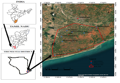 Figure 1a: Study area location map.

• Data 

The primary data location is shown in Figure 1b. The water levels from an open well and a bore well were checked every fifteen days. The Wenner (2-profile) and Schlumberger electrode arrangement (12 VES) methods were employed to acquire resistivity data. 100 total magnetic data points were gathered from the study region at a grid of 300 m x 300 m, as shown in Figure 2. Lithology information was gathered from the open well and bore well already on or near the site. The artificial recharge well in Ayyankulam is shown in Figure 3. The well is 3 m in length and 2 m in width (rectangular well). The system tank for the Nambiyar subbasin is the Thangamalpuram tank. It is the tank for the nearby recharge well, and both are connected through a canal. The canal is 1.5 m deep and 3 m wide. 1.2 to 1.5 m³/sec of water have flown into this well in 50 days. 

The Figure 4 shows the subsurface lithological information and sample at nearby VES 6. Hard rock formations are available on the north and north-eastern sides of the open well, as confirmed by lithology. Similarly, limestone formation is available on the south and south-western sides, and through the open well and bore well information, it is confirmed.

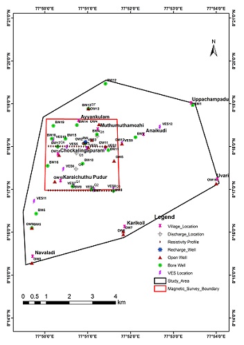 Figure 1b: Primary data illustrating the study area.

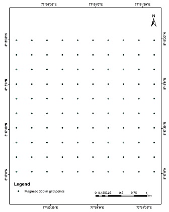 Figure 2: Grid point survey for Magnetic survey along the study area.

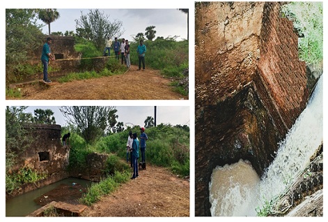 Figure 3: Artificial Recharge System at Ayyankulam Well.

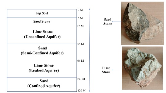 Figure 4: Lithology of the study area.

• Magnetic Method 

Magnetic Survey

A magnetic survey is a procedure that uses a magnetometer to measure the geomagnetic field over a certain area. Surveys document the spatial variation in the strength of the Earth's magnetic field. They may measure the total magnetic field strength using two geographically separated sensors, or they may measure the gradient of the magnetic field using two spatially separated sensors. In order to create a grid of data points, the magnetic measurements are made using magnetometers along profiles or a set of parallel profiles. This technique is often employed in magnetic surveys. A proton precession magnetometer was used to collect magnetic data from 100 sites in the study region (Table 1). The magnetometers used have the same sensitivity. For measuring diurnal variation, one is fixed at the base station, and the other is fixed in the research region for the survey. A certain time interval can be chosen for the base station magnetometer to record. Crosschecking the readings from the two magnetometers in the same location and at the same time for identical values is essential before moving further with the research. An east-west alignment is used for the sensor head. Every 10 minutes, base station readings are recorded. The stations should be placed far from any large metallic objects (such as reinforced concrete walls, electrical lines, cars, and metropolitan areas), as these objects might occasionally prevent data from being available within the survey grid in ground magnetic surveys. The range of the sources and the area to be examined are key factors in station separation. At any given time, three readings should be recorded there. Measurements must be taken until the difference between these three readings is within two gammas. The time of recording is also indicated because it will be necessary to account for diurnal variations. The main drawback of a ground magnetic survey is how challenging and time-consuming it is. High data resolution is a benefit, and field correction of survey data errors is also possible. Without processing, the magnetic data cannot be utilised. In general, it has been discovered that the processed findings acquired are well correlated with geological features. The International Geomagnetic Reference Field (IGRF) anomaly map was produced after the data underwent the necessary modifications, such as diurnal variations. 

 Table 1: Magnetic field data along the study area.

• Resistivity Method

Resistivity Survey 

Wenner electrode arrangement 

The Wenner array is made up of four collinear, equally spaced electrodes, as depicted in Figure 5. Typically, the outer two electrodes are current (source) electrodes, while the inner two electrodes are potential (receiver) electrodes. While maintaining an equivalent spacing between each electrode, the array spacing expands around the array midpoint. The Wenner array is also extremely sensitive to near-surface homogeneities, which can skew deeper electrical responses. Two profiles were conducted in this investigation. The readings are taken from west to east.

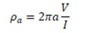 Where, ρ_a is apparent resistivity; it is electrode spacing; V is voltage in volts and I is current in amperes.

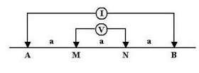Figure 5: Schematic diagram of Wenner method.

Schlumberger electrode arrangement

The Figure 6 depicts the Schlumberger array, which consists of four collinear electrodes. The two outer electrodes are current (source) electrodes, while the two inner electrodes are potential (receiver) electrodes. The potential electrodes are installed in the centre of the electrode array with a small spacing, usually less than one-fifth the spacing between the current electrodes. During the survey, the current electrodes are separated further, while the potential electrodes remain in the same position until the observed voltage becomes too small to measure. Typically, the current electrodes are expanded six times every decade.

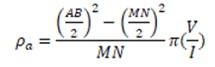Where, ρ_a is apparent resistivity; AB is current electrode spacing in meter; MN is potential electrode spacing in meter; I is current in amperes and V is voltage in volts. 

In this investigation, VES was conducted at 12 points spread over the area of the recharge well. The resistivity field data collection is shown in Figure 7.

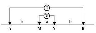 Figure 6: Schematic diagram of Schlumberger method.

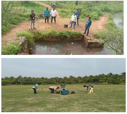 Figure 7: Resistivity field survey with M.Sc. Students in the month of January 2022.

• Water Level Indicator

A calibrated wheel attached to the counter mechanism of a water level indicator or dip metre is lowered into the well over a sensor attached to the end of a rope wound on a winch. On the winch, a panel metre shows full deflection and makes a buzzing sound when the sensor makes contact with the water's surface. The distance from the ground to the water level can be determined using a metric scale on the counter. It may be used to assess the water level in both open wells and bore wells, and it is simple to use. There were 15 open wells and 19 bore wells that were monitored every 15 days.

• Magnetic data analyses 

It is necessary to do magnetic data reduction to eliminate all sources of magnetic fluctuation from the observation other than those brought on by subsurface magnetic influences. Two corrections were made in this study, including a diurnal correction and an International Geomagnetic Reference Field (IGRF) correction. 

• Total magnetic field 

The magnetic or absolute value, of the magnetic field vector as displayed in Figure.8 is the magnetic total field. The magnetic total field, which is measured in units of nanotesla, describes the strength or intensity of the magnetic field (nT) (Figure 8).

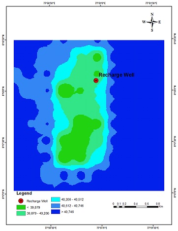 Figure 8: Spatial variation of Total Magnetic Field.

• IGRF Correction 

The geomagnetic correction is the magnetic equivalent of the latitude correction in gravity surveying, and it removes the effects of a geomagnetic reference field from survey data. The most exact approach to geomagnetic correction is the use of the International Geomagnetic Reference Field (IGRF), which represents the undisturbed geomagnetic field in terms of a large number of harmonics and incorporates temporal components to account for secular variation, as shown in Figure 9. Due to the IGRF's complexity, corrective measures must be calculated using a computer. It should nonetheless be highlighted that the IGRF is flawed because the harmonics employed are based on data from a sparse collection of scattered magnetic observatories. As it extrapolates the spherical harmonics obtained from observatory data forward, the IGRF is also prognostic. As a result, the IGRF can be drastically off in locations far from observatories. A magnetic field's components and values can be used to approximate the geomagnetic reference field. In this case, the IGRF value average of X, H, and F components, such as 40750 nT, was used. The Figure 10 depicts the spatial IGRF variation map.

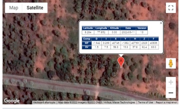 Figure 9: IGRF value of study area.

Source: http://www.geomag.bes.ac.uk/models_compass/igrf_calc.html

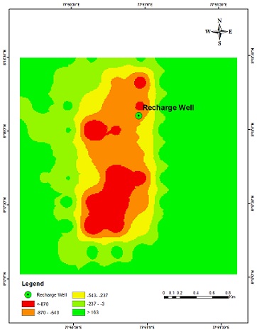 Figure 10: Spatial variation of IGRF Correction.

• Diurnal variation correction 

The effects of diurnal variation can be removed using a variety of techniques. Based on the time of observation, the variations in the base values are spread across the readings at stations taken over the day. The map of the spatial diurnal correction is shown in Figure 11. Based on the magnetic survey, it was possible to see a pattern where a very low magnetic field was taken into account as a very highly discontinuous karstic feature, or a very high degree of solution opening, which was then possibly followed by a highly discontinuous karstic feature, or a high degree of solution opening. Additionally, there are numerous abandoned bore wells in this region, which can lead to two outcomes: first, highly to very highly discontinuous groundwater, and second, deeper vertical groundwater flow.

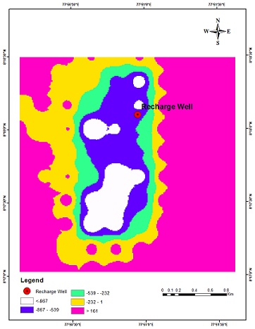 Figure 11: Spatial variation of Diurnal correction.

• Resistivity Data Analyses

Wenner method 

In this investigation, two lateral resistivity variations were found: one was close to the recharge well and the other was farther away; both were in west-to-east orientation. In this profile line one, certain resistivity smooth values are obtained between 400 and 1000 metres, which is a roughly discontinuous area. Additionally, a slight rise was seen on the second profile line at 500 and 1500 metres, signifying the potential location of bore wells, as shown in Figure 12.

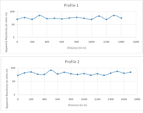 Figure 12: Horizontal variation of resistivity (Profile 1 & 2).

Schlumberger method 

In total, 12 vertical electrical sounding (VES) (Table 2) locations were investigated. The percentage relative root mean square (RMS) errors and interpretive models for each VES station provide a quantitative assessment of the method's quality. The number of layers encountered in soundings ranged from two to three.

Table 2: Geo-electrical Parameters of Vertical Electrical Sounding points.

Qualitative Interpretation of VES Curves

In the qualitative interpretation approach, the number of layers and their resistivity are calculated using the field curve's shape as a guide. It provides details on the number of layers present, their continuity over the entire region, and the degree of homogeneity or heterogeneity present in each layer. The field resistivity sounding curves with two and three layers in the research area are shown in Figures 13a&b. This graph mostly contains H-type curves. The possible groundwater indication in the study area is reflected in it.

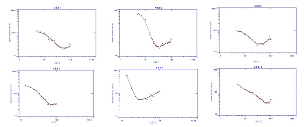 Figure 13a: VES curves from VES 1 to VES 6.

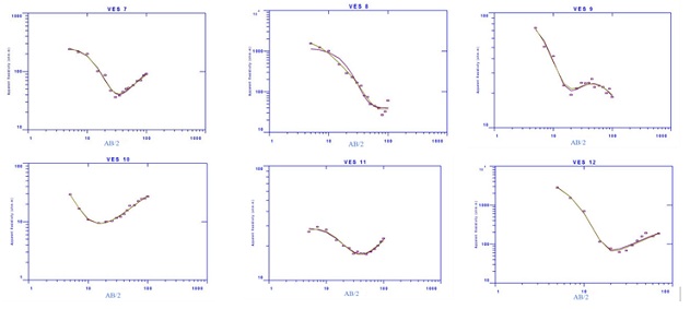 Figure 13b: VES curves from VES 7 to VES 12. 

Quantitative interpretation of VES

To validate the findings, the quantitative interpretation of the VES curve was connected and compared with the lithology based on the existing open well depth. The VES and lithology data match quite well up to this depth, as shown in Figure 14. Each layer's resistivity range and layer thickness (quantitative information) were found and are shown. VES 8 got a minimum of two layers, while VES 6 and 9 got a maximum of four layers, with the remaining layers all being three. The Figure 15a shows the spatial map of resistivity and layer thickness. The variation in the top layer of soil is shown on the layer 1 resistivity spatial map. Seashore sand and Aeolian soil both have resistivities that are greater than 400 ohm-m. A resistivity value of less than 50 ohm-m is produced by the clay type. In contrast to sandy clay, which produces values between 200 and 400 ohm-m, silty clay produces values between 50 and 200 ohm-m. Greater depth was found on the southern side of the recharge well, where the thickness of layer 1 varied from less than 5 to more than 11 metres. In the study region, different colours depict changes in layer thickness. 

Resistivity from the second layer was similarly divided into five groups. This was found to be less than 10 ohms in clay formation. In sandstone formations, 10 to 40 ohms were noted. Over 40 ohm-m indicates the presence of weathered sandstone. The second layer's thickness was determined to be deeper in the south-west direction. The eastern side has the lowest layer thickness. Resistivity spatial variation was only displayed in the third layer, as shown in Figure 15b. In this map, the calcareous limestone formation is under the recharge well and in the nearby south region (dark blue). But the hard rock formation is to the east of the recharging well (dark blue) (greater than 800 ohms). Due to deep bore wells and abandoned bore wells, the solution opening extends in green and yellow (from less than 100 ohm-m to 400 ohm-m). 400 ohm-m to 800 ohm-m was seen in limestone regions that had little erosion.

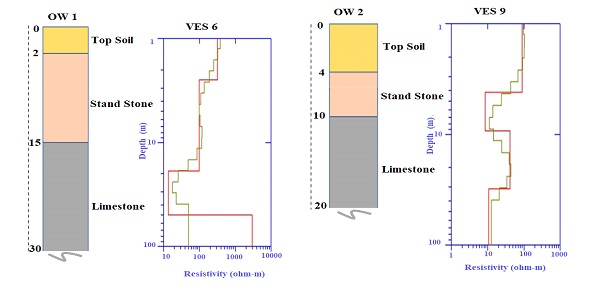 Figure 14: Correlation of subsurface geology with resistivity depth profile at VES 6 & VES 9.

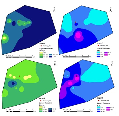 Figure 15a: Spatial Resistivity variation and Thickness variation of layer 1 & 2.

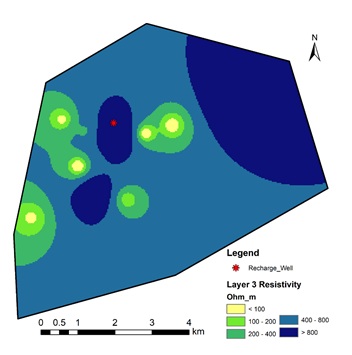 Figure 15b: Spatial variation of Resistivity of layer 3. 

• Spatial Groundwater fluctuation mapping 

 A spatial groundwater fluctuation map of an open well for various time steps in mean sea level (msl) is shown in Figure 16. There are five different categories on this map. It is rather obvious that the forms of the nearby recharge wells vary continuously every fifteen days. An open well's water level is a dynamic representation of shallow aquifer groundwater storage. Irrigation tanks and infiltration techniques can refill shallow aquifers. However, the input from the recharge well abruptly stopped, causing the water levels in the nearby monitoring wells to plummet as a response. The Figure 17 displays a groundwater bore well fluctuation map for a number of time steps in mean sea level (msl). On this map, there are five different categories. The patterns of the neighbouring recharge wells are constantly fluctuating every 15 days, which is highly obvious. The fluctuating water level in the bore wells represents semi-confined or confined aquifer groundwater storage. Semi-confined and confined aquifers can be filled by vertical flow (leakage) from shallow aquifers and abandoned bore well systems as shown in Figure 18. However, when the recharge well's input abruptly stopped, the water levels in the monitoring wells dropped as a result.

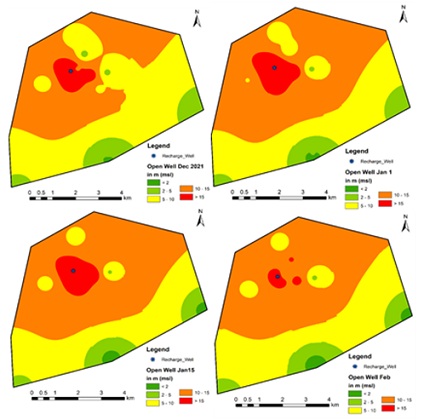 Figure 16: Spatial maps of Open well groundwater level at various time steps. 

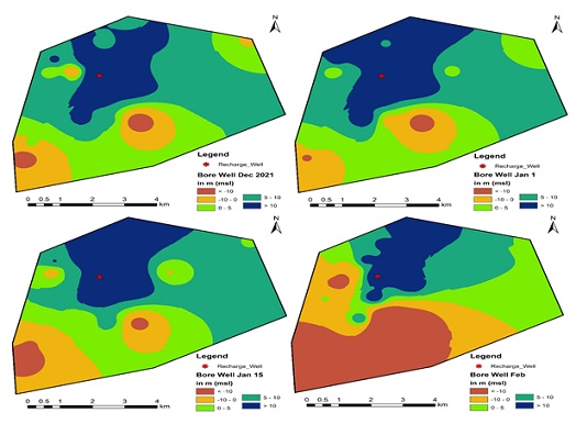Figure 17: Spatial maps of bore well groundwater level at various time steps.

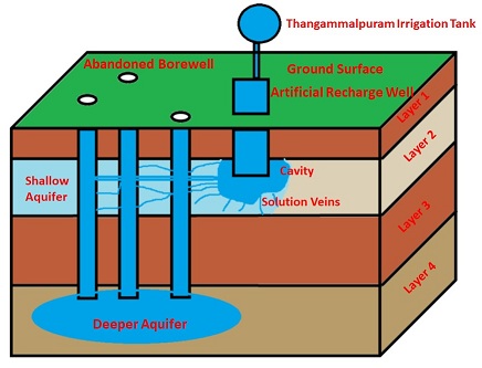 Figure 18: 3D view projection of Ayyankulam Recharge well system.

• Discharge

The Table 3 displays the various locations in this study area where bore well discharge was measured. Most of the time, it is used for irrigation for 5 to 10 hours, occasionally longer. However, Q1, Q4, and Q5 values above 13 m³/hr suggest some relationship between the bore well and the recharge well. When the inflow to the Q6 recharge well was interrupted, it no longer functioned as a potential well, and the water level dropped. Hard rock terrain had a flow rate of less than 1 m³/hr. 

Table 2: Pumping rate at the study area.

In this study, the water flow direction of a recharge well was identified using the magnetic method, a resistivity metre, and a water level indicator. The Ayyankulam recharge well receives water from the Nambiyar canal and Thangammalpuram irrigation tank. The magnetic method's results indicate a south-to-southwest direction of flow. Also, the resistivity method gives a similar direction of flow, but in this result, some quantitative depths are observed in the same directions. Twelve VES were performed to study the aquifer's structural and hydro-geophysical settings. The most common recorded curve type was an H-type curve. The main water-bearing layer was considered to be saturated unconsolidated sedimentary (sand) in the deeper aquifer (confined aquifer) and shallow sandstone/limestone aquifer (unconfined aquifer), and their resistivity values were calculated. From December 2021 to February 2022, groundwater levels were measured on a regular basis with a water level indicator. Readings were taken from both bore wells and an open well that are present in and around the Ayyankulam recharge well, i.e., approximately 45 km², using a water level indicator. In this study area, the groundwater level fluctuated between 5 and 10 m (msl). Throughout the region, water is used for domestic and agricultural purposes. The presence of an unconfined aquifer flow in the southwest direction was found in the survey. However, to the south and southwest of the recharge well, some abandoned bore wells are not in use because they were filled with a solution of weathered limestone or sand, and some bore wells are still working properly. These bore wells aid in recharging the deeper aquifer. It is water from the recharge well that accelerates the recharge of confined aquifers via bore wells to the south. From the pumping tests conducted, it is found that groundwater discharge from the pumping well near VES 7 may take 14 cubic metres of water per hour in this research region, but groundwater discharge from the pumping well near VES 8, which is to the southeast of the recharge well, can take only 0.72 cubic metres of water per hour. Deeper aquifer recharges from the Ayyankulam recharge well have been found in the VES 7 area. This implies that the water is pouring through the Ayyankulam recharge well from the south and southwest directions. 

The study region is considered as soft rock zone because of the resistivity high limited up to 250 Ωm. below the top layer the intermediate resistive layer is observed with 70 Ωm as average resistivity and that can be interpreted as stiff kaolinite clay layer. Wherever the laterite patch is, absent in that places clay layer is observed that can be delineated based on the lateral resistivity variations between the consecutive sounding points. Thus whenever the dissolution canal dimension is increased it is capable to discharge huge amount of fresh water collected and accumulated from all the vein formations. If properly planned, this karst water can be utilized for satisfying public water needs and for irrigation because already the region facing severe water crisis is summer.

• The study will reveal the natural recharge system relevant with lithological characterization to quantify the Groundwater system at each location along the study area. It will discriminate and evaluate the rate of improvement for groundwater quality in particular area. 

• The data on rain water supply and create the natural recharge system in particular area will be useful to assess the erosion pattern in subsurface lithological pattern and to identify the impact of sea-water intrusion in coastal regions. 

• This interpretation will be an eye-opener to understand the natural recharge system in other similar areas in Tamilnadu.

I wish to thank Dr. S.Rajakumar, Mr. S Suriyarajan, Mr. J Vignesh, Mr. J S Jhon Algin, and Mr. Ahamed Kabeer Rahmathullah, M.Sc. graduate students from the Centre for Geotechnology, Manonmaniam Sundaranar University, Tirunelveli, for their support in collecting high-quality field data during the field survey. I would also like to thank the registrar of M.S. University for allowing me to do this research independently.

1. Srinivasan V (2022) IIT Madras Researchers Propose Rapid Groundwater Recharge technology near Ayankulam village of Tirunelveli for combined flood and drought mitigation. Retrieved in Online.
2. White WB (1988) Geomorphology and Hydrology of Karst Terrains: New York. Oxford University Press, P: 464.
3. Bakalowicz M (2005) Karst groundwater: a challenge for new resources. Hydrogeology Journal. 13: 148-160.
4. Ford D, Williams P (2007) Karst Hydrogeology and Geomorphology. Chichester, England, Wiley. P: 562.
5. Goldscheider N, Drew D (2007) Methods in Karst Hydrogeology. London Taylor & Francis. International Contributions to Hydrogeology. 26: 264.
6. Sowers G (1996) Building on Sinkholes: Design and Construction of Foundations in Karst Terrain. New York, NY: ASCE Press.
7. Ram Das D (2011) “Site Evaluation Report, Kudankulam Nuclear Power project unit 3 to 6”.
8. Stewart M, Layton M, Lizanee T (1983) Application of resistivity surveys to regional hydrogeologic reconnaissance. Groundwater, 21: 42-48.
9. Anisimova VO, Koronovsky NV (2007) Lineaments in the central part of the Moscow Syneclise and their relations to faults in the basement. Geotectonics, 41: 315-332.
10. Kumar NK, Aiyagari N (1997) Artificial recharge to groundwater.
11. Cheng Q, Chen X, Tao M, Binley A (2019) Characterization of Karst structures using quasi-3D electrical resistivity tomography. Environ. Earth. Sci. 78: 285.
12. Tao Z, Cui Z, Yu J, Khayatnezhad M (2021) Finite difference modelings of groundwater flow for constructing artificial recharge structures. Iran. J. Sci. Technol-Trans. Civ Eng. 46: 1503-1514.
13. Hao S, Li F, Li Y, Gu C, Zhang Q, et al. (2019) Stable isotope evidence for identifying the recharge mechanisms of precipitation, surface water, and groundwater in the Ebinur lake basin. Sci. Total. Environ. 657: 1041-1050.
14. Demlie M, Wohnlich S, Wisotzky F, Gizaw B (2007) Groundwater recharge, flow and hydrogeochemical evolution in a complex volcanic aquifer system, central Ethiopia. Hydrogeol. J. 15: 1169-1181.
15. Smerdon BD, Gardner WP (2022) Characterizing groundwater flow paths in an undeveloped region through synoptic river sampling for environmental tracers. Hydrol Process. 36.
16. Woldeyohanners YY, Nzikou M (2018) Application of airborne geophysics and geochemistry to characterize groundwater flow path. Geotech. Geol. Eng.
17. Bishop JM, Glenn CR, Amato DW, Dulai H (2017) Effect of land use and groundwater flow path on submarine groundwater discharge nutrient flux. J. Hydrol. Reg. 11: 194-218.
18. Quiroz Londoño OM, Martínez DE, Dapeña C, Massone H (2008) Hydrogeochemistry and isotope analyses used to determine groundwater recharge and flow in low-gradient catchments of the province of Buenos Aires, Argentina. Hydrogeol. J. 16: 1113-1127.
19. Reynolds R, Rosenbaum JG, Hudson MR, Fishman N (1990) Rock magnetism, the distribution of magnetic minerals in the Earth’s crust, and aeromagnetic anomalies, in W. F. Hanna, ed., Geologic applications of modern aeromagnetic surveys: U.S. Geological Survey Bulletin. 1924: 24-45.
20. Tafila O, Ranganai RT, Moalafhi DB, Moreri KK, Maphanyane JG (2022) Investigating groundwater recharge potential of Notwane catchment in Botswana using geophysical and geospatial tools. J. Hydrol. Reg. 40: 101011.
21. Furlan L, Rosolen V, Sales J, Moreira CA, Ferreira ME, et al. (2020) Natural water storage and aquifer recharge assessment in Brazilian Savanna wetland using unmanned aerial vehicle and geophysical survey. Authorea.
22. Gaber A, Mohamed AK, ElGalladi A, Abdelkareem M, Beshr AM, et al. (2020) Mapping the groundwater potentiality of west Qena area, Egypt, using integrated remote sensing and hydro-geophysical techniques. Remote. Sens. 12: 1559.
23. Pepin K, Knight R, Goebel M, Kang S (2022) Managed aquifer recharge site assessment with electromagnetic imaging: Identification of recharge flow paths. Vadose Zone J; 21.
24. Hasan M, Shang Y, Jin W, Akhter G (2021) Joint geophysical prospecting for groundwater exploration in weathered terrains of south Guangdong, China. Environl. Monit. Assess. 193.
25. Meneisy AM, Al Deep M (2021) Investigation of groundwater potential using magnetic and satellite image data at wadi el Amal, Aswan, Egypt. Egypt. J. Remote. Sens. Space. Sci. 24: 293-309.
26. Oni AG, Eniola PJ, Olorunfemi MO, Okunubi MO, Osotuyi GA (2020) The magnetic method as a tool in groundwater investigation in a basement complex terrain: Modomo Southwest Nigeria as a case study. Appl Water Sci. 10.
27. Parsekian AD, Regnery J, Wing AD, Knight R, Drewes JE (2014) Geophysical and Hydrochemical identification of flow paths with implications for water quality at an ARR site. Ground water. Monit. Remediat. 34: 105-116.
28. Jiang X, Wan L, Wang J, Yin B, Fu W, et al. (2014) Field identification of groundwater flow systems and hydraulic traps in drainage basins using a geophysical method. Geophys. Res. Lett. 41: 2812-2819.
29. Meyerhoff SB, Maxwell RM, Revil A, Martin JB, Karaoulis M, et al. (2014) Characterization of groundwater and surface water mixing in a semiconfined Karst aquifer using time-lapse electrical resistivity tomography. Water. Resour. Res. 50: 2566-2585.
30. Mogaji KA, Lim HS, Abdullah K (2015) Modeling of groundwater recharge using a multiple linear regression (MLR) recharge model developed from geophysical parameters: A case of groundwater resources management. Environ. Earth. Sci. 73: 1217-1230.
31. Robert T, Caterina D, Deceuster J, Kaufmann O, Nguyen F (2012) A salt tracer test monitored with surface ERT to detect preferential flow and transport paths in fractured/karsticfied limestones. Geophysics. 77: B55-B67.
32. Somaratne NM, Mann S (2016) Integrated use of geological, geophysical, radiocarbon and stable isotopes data for tracing the conduit flow paths in a small karstic aquifer: Poocher swamp freshwater lens, South Australia. Environ. Nat. Resour. Res. 6: 119.
33. Redhaounia B, Ilondo BO, Gabtni H, Sami K, Bédir M (2016) Electrical resistivity tomography (ERT) Applied to Karst carbonate aquifers: Case study from Amdoun, Northwestern Tunisia. Pure Appl Geophys. 173: 1289-1303.
34. Ravindran AA,Venkatesh K, Durai ED (2012) “Characterization of the Geology and subsurface limestone crystalline mining using 2D ERI at Puthur mines,Tirunelveli,Tamilnadu”. Archives of Applied Science Research. 4: 1261-1265.
35. Daesslé LW, Pérez-Flores MA, Serrano-Ortiz J, Mendoza-Espinosa L, Manjarrez-Masuda E, et al. (2014) A geochemical and 3D-geometry geophysical survey to assess artificial groundwater recharge potential in the Pacific coast of Baja California, Mexico. Environ. Earth. Sci. 71: 3477-3490.
36. Pradeepa F, Shaji JP, Rajkumar S, Arunbose S, Srinivas Y (2018) Delineation of Aquifer flow using electrical geophysical method in Aayankulam-Radhapuram which shows exceptional drainage and flow pattern, International journal of basic and applied research. 8: 1228-1236.
37. Sun H, Cheng M, Su C, Li H, Zhao G, et al. (2017) Characterization of shallow Karst using electrical resistivity imaging in a limestone mining area. Environ. Earth. Sci. 76.