Regression Pluviometry- Morphometry

We present a network of rainfall stations unevenly distributed in the study area. In each of the stations, we have estimated certain rain-related parameters. Each of the letters is related to a variable distributed at the station, according to a given probability law of central value equal to the estimated parameter. The error resulting from parameter estimation will be inversely proportional to the square root of the sample size. This will be a sampling error and will not be the only error in the study. In fact, the identification of each law of probability is made up of a sample in which each element is measured with a certain error. The main goal is to be able to connect, following a linear model, the rain-related parameters to other relief-related parameters. The relief-related parameters, which would affect the rain are themselves variable for each station. In the framework of the model, they will be assumed without any error (this hypothesis is employed for model simplification).

The main idea is to map the characteristics fields of precipitation taking into account as much information as possible. The first information is without a doubt the point estimates (punctual estimates) of extreme rainfalls for the different time laps. We seek to know the number of parameters that can characterize the site and to find out if there are any other parameters that can affect the distribution of precipitation: the altitude of the precipitation station, the longitude measured by x Lambert, the latitude measured by y Lambert, the altitude averaged over a number of fixed DTM nodes closest to the station [1-5]. 

Precipitations can therefore be considered as a function of three components: 

R(x)=f(Rsite(x),Rsituation(x), Rrégion(x))

The work consists of identifying site specific characteristics and parameters that vary too quickly to be mapped from punctual rainfall point measurements only. The only features of the region are of course the x_j and the y_j

We consider as explanatory variables the main components of the relief cp1,...cp10, which are only calculated at the rainfall stations for a DTM step of 2 km. From a numerical terrain model whose step = 2 km applied to our field of 250km/450km let it be a matrix of altitudes of 225 lines and 125 columns, we seek to calculate the principal components of the relief while taking into consideration the effect of a pluviometric buffer zone of a radius of 4 Km which equates a radius of 4 meshes and hence rendering the landscape surrounding the point "o" as a matrix (9 * 9) of mean altitudes and this site will be characterized by altitudes at the level of the 81 nodes of the mesh and thus by 81 values. 25389 sites in the French Alps area can be characterized from the DTM (excluding the 4 most eastern columns, the 4 most westerly columns, the 4 southernmost lines and the 4 most upright lines north wards).The application of the PCA to the z-matrix (25389.81) shows the following results: 

The first 8 main components account for more than 90% of the field variance (85% for the top 5)

From the figure log(λk) = f(k) we see that only 6 components are sufficient to summarize the relief. 

Each vector a_ik appears as a basic landscape and are very clear. 

• α i1: stacking effect (35% of variance explained)
• α i2: presence of a north-west/south-east slope (22% explained variance)
• α i3 presence of a south-westerly/north-easterly slope (18% variance explained)
• α i4: Collar effect (6% of explained variance)
• α i5: Collar effect(4% of variance explained)
• α i6: unclear effect
• α i7: unclear effect
• α i8: unclear effect
• αi₂: cash-in effect (35% explained variance)
• αi₂: presence of a Northwest / South East slope (22% explained variance)
• αi₃ has a southwest / northeast slope (18% explained variance)
• α i₄: neck effect (6% explained variance)
• αi₅: neck effect (4% explained variance)
• αi₆: unclear effect
• αi₇: effect unclear
• αi₈: effect unclear 

We have reported the eight fields of αi1, αi2, α i3, αi4, αi5, αi6, αi7, αi8 illustrated by the first eight principal components of the relief. The site environment is a linear combination of these eight basic "landscapes". These basic landscapes are plotted on a surface grid (8 * 8) km and not equal to 2 km and whose basic data are the relative altitudes calculated at the 24 nodes of the grid relative to the central node. Basic Landscape # 1 illustrates the existence of a depression or summit around the central point. Landscape # 2 has a downward slope to the northwest or a downward slope to the southeast. The third landscape shows a slope either descending northeast or south-east direction northwest, the fifth landscape also shows “Collar effect” but direction is east-west or north-south. Basic Landscapes No. 6, 7, 8 reveal finer spatial structures not easy to interpret (Figure 1).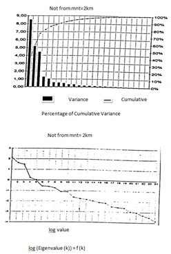 

Figure 1: Basic Land scapes n 6,7,8 reveal finer spatial structures not easy to interpret not from mnt=2km.

After a long reflection on the problem of the relationship between the characteristics of the extreme rainfall and the relief in this region, we thought that it could be the look of the alpine chain that draws elliptical arcs like structure extending from the Mediterranean to the west to reach as far as the Jura in the east, that may be of importance, hence we said to ourselves that the characteristics of the extreme rainfall events are related to the distance separating a given station from the two foci of an ellipsoid having the same aspect as the chain, therefore we traced by hand an elliptical arc having the shape of the chain, from a dozen points taken on this arc, we looked for these two foci which are f1 (x = 950 km, y = 240km) f2 (x = 1025, y = 450km). The new variable to introduce in the regression’s equation is the distance of each station to the two foci (figure 2 and 3) and that we shall note "dist".

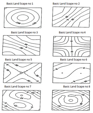 Figure 2: Eigen vectors of the basic landscapes on the area of 8*8km. 

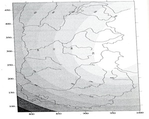Figure 3: The Distance Variable.

I = a / t^b

X = I * t = (a / t^b) * t = a * t^(1-b) = a * t^n₁ = (x₀ + g^*u)^* tⁿ

I: Rainfall intensity

A: Rain for a return period and a given duration

Finally we may write,

X (t, T) = [ x₀ (x+y) + g (x,y)^*u (T) ]^* t^n(x,y)

x₀: Position parameter

g: Gradex

u: Gumbel reduced variable

n: Montana parameter

t: Time laps

T: Return periods 

Knowing the map x₀, the grade X and the Montana parameter we can determine the value of the rain for any time laps and any return period and at any place of the domain, hence we decided to trace three cards (x₀ (x, y), g (x, y) and n (x, y)), at the beginning we took the time step of 1h and the grade X was calculated for the return periods of 20 years and 100 years.

g(1h) = [x(100 years) - x(20 years) ] / [u(100 years) - u(20 years)]

For the Montana parameter we took a mean value between the one calculated for T = 20 years and T = 100 years, which we called n_moy.

n_moy = (n(20 years)+n(100 years))/2

n(20 years) :Montana parameter calculated for rainfall of 20 years

n(100 years) :Montana parameter calculated for rainfall of 100 years

And x₀ will be the rain for T = 20 years and t = 1h and we note x (1h, 20 years) 

We sought the regression between x (1h, 20years), g (1h), and n_moy and the different explanatory variables, namely the main components of the relief, the regional parameters, the altimetry parameters and the distance

from the ellipse foci. We find as results:

x (1h,20years)=8.31*10^-2 X -3.05*10^-2 Y+0.112629 dist-77.29678

R=80.68%

g (1h)=1.51*10^-2 X - 8.21*10^-3 Y+2.32*10^-2dist - 13.19608

R=72.95%

n_moy= 1016*10^-4 Z+0.29048

R=59.34%

We conclude that for the rain x (1h, 20 years), the more we get deeper into the chain (the distance to the foci increases) the more it rains, the altitude does not intervene and this is explained by the fact that the rain is of a stormy type, that is to say that the convective motions of humid air masses causing thunderstorms are, indeed not a priori related to the study of the pluviometric stations. For the hourly Gradex we also note that the deeper we go into the chain the higher the Gradex, and the term altitude does not intervene. On the other hand, the Montana parameter is explained using a single variable, which is the altitude, and which has a positive sign meaning that this parameter is strong on the bumps and weak in the hollows. After having drawn the maps of the hourly rain of 20 years and that of the grade X we conclude that they have a very smooth shape and that was already predictable; we preferred to work on other time lapses where the altitude could play a role and it was thought that it would be better to consider the rain and the grade X for the lap of 24 hours. 

We find the following regression equation:

x (24h,20years)=0.271666 X -7.62*10^-2 Y+2.28*10 ^-2 Z +0.32137 dist-248.3298

R=62.33%

g (24h)=0.5636*10^-1 X –0.2455*10^-1Y+4.0862*10^-3dist–50.49

R=61.81%

It's the variables of latitude, longitude and distance to foci that best explain the 20-year hourly rainfall with a multiple correlation coefficient of 0.807 (Tables 1 and 2). If we look at the partial correlation coefficients, we find that the distance variable has the largest coefficient of the order of 0.754, while that of the other two explanatory variables latitude and longitude does not exceed the value of 0.5 in absolute value (respectively -0.506 and 0454), we conclude that it rains more on the outer slopes of the Alps directly exposed to humid air masses. The variable altitude does not intervene regardless of the altitude of the post or the surrounding altitudes what is explained by the fact that this rain is of the storm type provoked by the stacking of the valleys favoring the descent along the high reliefs. For the hourly grade X the regression equation allows us to reach a value of correlation coefficient of the order of 0.7295 but which remains less than that of the r hourly 20 year rain. They are the same explanatory variables that appear in the same order and with the same sign: the longitude first with a positive sign, then the latitude with a negative sign and the distance in third position with a positive sign. The latter has the highest partial correlation coefficient (0.629) which is about twice that of longitude (0.3346), and much larger than latitude (-0.5175), meaning that the effect of distance to foci is the most important and therefore the more one goes deeper into the chain in the direction of the west the higher the grade X (Tables 3 and 4). For the 20 year old rain, in addition to the usual variables a variable that appears which the altitude, with a positive sign is, it ranks in third position after the longitude and the latitude. All variables have positive sign regression coefficients except latitude. The partial correlation coefficient of the distance variable decreases (0.5) compared to that of the hourly 20 year rain, which is recovered by the effect of the altitude whose partial correlation partial reaches the value of 0.3658. The latitude and longitude variables retain their partial correlation coefficient value. We conclude that the deeper we go west in the chain the more this rainfall parameter is plentiful, especially on the bumps than in the hollows .For the daily gradex we find the appearance of the altitude variable to be compared with the hourly grade X, the multiple correlation coefficient has decreased (0.62) the partial correlation coefficients of the different variables (longitude, latitude and distance) have decreased, as for the 24 hours 20 year rain, the appearance of the altitude effect reduced the effects of the other variables, although the effect of distance remains in the lead with a partial correlation coefficient of 0.4287 (Tables 5 and 6). The daily grade X increases moving further east to west, especially as the altitude becomes higher. The only explanatory variable of this parameter is the altitude with a positive sign. The coefficient of multiple correlations is of the order of 0.5934 meaning that this parameter is strong on the bumps and weak in the hollows [6-10] (Figures 4-7). 

Table 1: Regression of pluviometric variables. 

Table 2: Hourly rainfall for 20 years. 

Table 3: Hourly Grade x. 

Table 4: Daily rainfall for 20 years. 

Table 5: Daily Gradex. 

Table 6: Montana.  

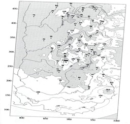Figure 4: Estimation of precipitation in 24 hours (T = 20 years pen mm). 

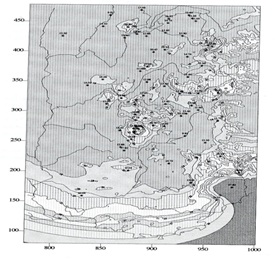Figure 5: Estimate of Grade X in 24 hours (mm). 

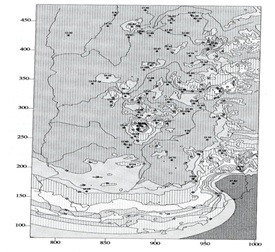Figure 6: Estimate of Grade X in 24 hours (mm). 

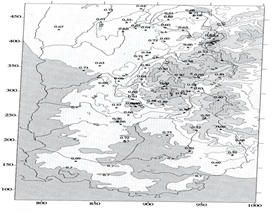Figure 7: Estimate of the Coefficient b Montana I (t) = a / t ^ b).

The principal components analysis shows that the space of the 19 rainfall parameters can be reduced to an equivalent space of dimension 2 and practically some is the dimension of the space of the parameters it is always reduced to a space in two dimensions provided that there is the Montana parameter. The space of the stations of dimension 50 is reduced to an equivalent space of dimension 5. Therefore the rainfall information observed on the 50 stations is equivalent to 2 rainfall parameters measured on 5 average stations each of which represents a class. The relief analysis shows that each landscape in the Alpine region is a combination of the six basic landscapes. The use of these landscapes in the rainfall-morphometric regression did not give spectacular results surely because the mesh of DTM is not sufficiently fine. It is the latitude, longitude, altitude of the rainfall post and the distance from the households that play the greatest role in this regression.

1. Benichou P, Lebreton O (1987) Takingin to account the topography for the cartography of statistical pluviometric fields Meteorology 7th series 19: 23-24.
2. Blanchet G (1993) variability of annualprecipitation in the Rhone-Alpes region: cartographic presentation 68:101-109.
3. Braud I (1990) Methodologicalstudy of principal component analysis of two-dimensional processes. Effect of numerical approximations and sampling and use for the simulation of randomfields: Application to the treatment of monthlysea surface temperatureson the intertropical Atlantic.
4. Creutin D (1979) Optimal interpolation method of hydrometeorological fields comparison and application to a series of Cévenol rainy episodes 63-64.
5. Desurosne I (1992) Rainfall intensity gradient in relief areas: experiments and first data modeling of an Alpine Rhône network, the TPG. »Thesis from Louis Pasteur University, Strasbourg.
6. Jean-Pierre L (1984) Data analysis and automatic cartography in hydrologyElement of hydrology Lorraine.Thesis State Doctorate, I.N.P.L. Nancy.
7. Jean-Pierre L (1982) Automatic mapping of rainfall characteristics: Taking into account the rainfall-morphometry relationships.
8. Obled CH (1979) Contribution to the analysis of data in hydrology: the prediction of accidental phenomena and the analysis of spatial fields" Thesis of spatial fields "State Thesis, U.S.M.G-I.N.P Grenoble.
9. Slimani M (1985) Study of rains of rare frequency withlow time steps in the Cévennes-Vivarais region: Estimation, relation with the relief and syntheticcartography. Doctor-Engineerthesis, I.N.P Grenoble.
10. Tourasse P (1981) Spatial and temporal analyzes of precipitation and operational use in a flood fore casting system. Application to the Cévennes régions. Coping with Floods 257: 473-501.