The Dynamics of the Euphrates River Water Level in Response to Dams: A Study of NDWI Index and Satellite Monitoring Using Advanced Statistical Methods

The Euphrates River, with a length of approximately 2,800 kilometers (some sources mention 3,000 kilometers), is one of the largest and most significant rivers in the Middle East [1]. It originates from the Anatolian Mountains in Turkey and flows through Syria and Iraq, eventually joining the Tigris River to form the Shatt al-Arab. The Shatt al-Arab, in turn, merges with the Karun River in Iran, forming the Arvand River, which finally discharges into the Persian Gulf. The Euphrates River holds particular importance for water supply, agriculture, fishing, hydropower generation, and the preservation of biodiversity and the historical identity between the Mesopotamian regions [2-6]. Studies have shown that the highest volume of river discharge occurs in the months of April and May, accounting for approximately 36% of the annual volume (sometimes reaching 60 to 70%) on average [7-9]. Prior to this study, researchers had warned about the hazards and consequences of uncontrolled dam construction in the Mesopotamian basin [10-15]. Construction and operation of numerous dams upstream of this river have had significant negative impacts on the water level, flow, and quality with Turkey taking the lead by constructing and operating 14 dams on the main branches and tributaries of the Euphrates [16-19]. The Atatürk Dam reservoir alone has the capacity to hold the entire annual discharge of the Euphrates River. Following Turkey, Syria has constructed 4 dams [20-23] and Iraq has also implemented 4 dams/flood barriers [24-32].

Research indicates that the hydrological regime and flow pattern of the region and this river have been altered, resulting in a decline in the stability of groundwater levels [33-35]. Furthermore, climate change has led to a reduction in precipitation and an increase in evaporation [36] within its watershed [37-40], although this is a global trend [41-45]. Wars, dam constructions, droughts, and mismanagement have caused significant fluctuations in the water level of the Euphrates River and its associated lakes in recent decades [46-50]. Ecological destruction and the loss of wetlands between the rivers, which were habitats for many species, are among the consequences of these dam constructions [51-55]. Additionally, the construction of these dams has put cultural and archaeological heritage at significant risk of destruction or even complete loss on a large scale [56-57].

To study the dynamics of water levels in the Euphrates River, it is necessary to employ effective and accurate methods. One commonly used approach for determining the water levels of rivers and lakes is the utilization of the Normalized Difference Water Index (NDWI). This hydrological index is derived from satellite imagery and indicates the extent to which the Earth's surface is influenced by water. By utilizing the NDWI, it is possible to determine the water levels of the Euphrates River and the Ataturk Dam Lake in Turkey, the Tabqa Dam in Syria, and the Ramadi Dam/Floodgate in Iraq, and compare them to the water level of the river in the vicinity of the Hira city, which is located in the province of Najaf before it joins the Tigris River.

This study aims to investigate the water level dynamics of the Euphrates River in response to the construction of numerous dams upstream. The main hypothesis of this research is that dam construction upstream of the river has led to a significant decrease in the water level of the river and changes in its hydrology. To evaluate this hypothesis, a combined approach of the NDWI index and satellite monitoring using advanced statistical methods has been employed [58-60]. In this method, the NDWI index has been calculated for four points from 2013 to 2022 using Landsat 8 satellite images. Subsequently, the fluctuations in the river water level have been examined using advanced statistical methods such as the Kolmogorov-Smirnov test, Shapiro-Walk test, histogram plotting, correlation analysis, coefficient of determination, and others. The following questions were addressed: 

1. Has the water level changed in the four study areas during the study period (2013-2022)?
2. If it has changed, what pattern is observed in the water level fluctuations?
3. What factors may have influenced the water level changes?

This research aimed to assess the water level changes in four geographical regions (Table 1) using Landsat 8 OLI/TIRS satellite images and the NDWI index. Satellite images with a spatial resolution of 30 meters and a temporal interval of 15 to 25 days were extracted for four UTM coordinates to analyze the NDWI index. This index is a spectral index used for water delineation and moisture detection, calculated using the green and near-infrared (NIR) bands [61-62]. The formula for the NDWI index is as follows:

Satellite images were downloaded from the United States Geological Survey and EOS Data Analytics systems, and the necessary information for each of the selected areas was collected from 2013 to 2022. Among the obtained images, 546 photos were downloaded with suitable quality and without clouds or shadows. The analysis and examination of the images and data were carried out in two stages. In the first stage, all images (from 2013 to 2022) were analyzed and examined. In the second stage, only the pictures from the month of August were investigated (2 images per month). The reason for selecting this month was the completeness of the collected data for each year in each of the studied coordinates. The geographical areas under investigation include:

Table 1: Geographical Specifications of the Study Points (Source: Current Research)

ENVI 5.3 software was used for satellite image processing, Microsoft Excel 2019 software was utilized for data classification, archiving, and table generation, SPSS 26 software was employed for statistical tests, data analysis, and table plotting, Microsoft Word 2019 software was used for manuscript writing, and EndNote 21 software was utilized for reference citation.

The study radius at each of the four points (Table 1) was 140 meters from the shoreline. This radius was determined based on the Cadmium method, which is a statistical approach for estimating the shoreline using the NDWI (Normalized Difference Water Index) index [63]. Initially, a reference line was drawn near the shoreline (separately for each coordinate). Then, using the NDWI index, water and land points were identified in each pixel [64-66]. Subsequently, an optimized algorithm was used to draw a new line that best matched the water-land interface, which was considered as an estimated shoreline. The Cadmium method utilizes several parameters to determine the appropriate radius and draw the reference line, which depend on the geographical conditions, season, tidal state, and image accuracy. One of these parameters is the spatial response width, which represents the distance between two points having the highest (water) and lowest (land) NDWI values. In this method, using multiple different images, the spatial response width was calculated for each area. The aim was to measure the magnitude of water level changes (water surface elevation).

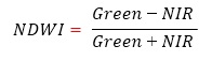
The normality test was conducted separately for the data obtained from each area. Therefore, the normality of the data for the first coordinate was assessed using the Kolmogorov-Smirnov test (Table 2) and by plotting a histogram (Figure 1). Since the calculated p-value was 0.200, which is greater than the significance level (α) of 0.05, and the histogram exhibited a bell-shaped distribution, the data were confirmed to be normally distributed. Consequently, parametric tests were employed for data analysis and examination. 

One-Sample Kolmogorov-Smirnov Test 

Average Variance 

Table 2: Normality Test for Data of the First Coordinate (Ataturk Dam) using the Kolmogorov-Smirnov Test (Source: Current Research)

a. Test distribution is b. Calculated from data. c. Lilliefors Significance Correction. d. This is a lower bound of the true significance.

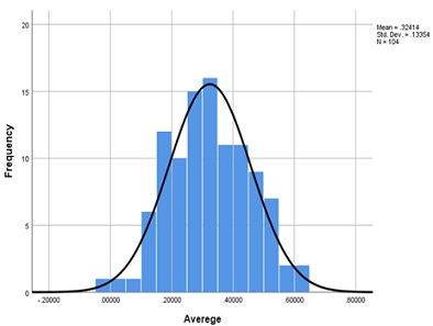
Figure 1: Histogram Plot for Assessing the Normality of Data for the First Coordinate (Ataturk Dam) (Source: Current Research) 

The normality of the data for the second coordinate was also examined. In the Kolmogorov-Smirnov test (Table 3), which is conducted using numerical calculations, the p-value was found to be 0.018 < 0.05 = α, indicating non- normality of the data. However, the histogram showed a bell-shaped distribution, indicating normality of the data (Figure 2). Therefore, a third test was conducted to verify the results of the previous two tests. In the Shapiro-Walk test (Table 4), the normality of the data was not confirmed, with a p-value of 0.013 < 0.05 = α. Hence, non-parametric tests were performed for the data obtained from the second coordinate.

One-Sample Kolmogorov-Smirnov Test

Average Variance

Table 3: Examination of Normality of the Second Coordinate Data (Tabqa Dam) using the Kolmogorov-Smirnov Test (Source: Present Study)

a. Test distribution is b. Calculated from data. c. Lilliefors Significance Correction. 

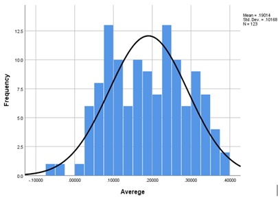Figure 2: Histogram for Assessing the Normality of the Second Coordinate Data (Tabqa Dam) (Source: Present Study)

Tests of Normality

Table 4: Assessment of the Normality of the Second Coordinate Data (Tabqa Dam) using Shapiro-Walk Test (Source: Present Study)

In the examination of the normality of the third coordinate data, the Kolmogorov-Smirnov statistical test (Table 5) and the histogram plot (Figure 3) were conducted. The normality of the data was confirmed in both methods, with a p-value of 0.200 < 0.05 = α, indicating that the data followed a normal distribution. Therefore, parametric tests were employed for subsequent analysis stages. 

One-Sample Kolmogorov-Smirnov Test

Average Variance

Table 5: Assessment of normality for the third coordinate data (flood barrier) using the Kolmogorov-Smirnov test (Source: Current Study)

a. Test distribution is b. Calculated from data. c. Lilliefors Significance Correction. d. This is a lower bound of the true significance.

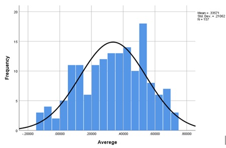Figure 3: Histogram chart for assessing the normality of the third coordinate data (Ramadi Flood Barrier) (Source: Current Study).

The normality of the fourth coordinate data was also examined. In the Kolmogorov-Smirnov test (Table 6), the normality of the data was confirmed (p-value = 0.200 < 0.05 = α). Additionally, the histogram chart (figure 4) further confirmed the normality of the data. Parametric tests were also used for this section.

One-Sample Kolmogorov-Smirnov Test

Average Variance

Table 6: Investigation of the normality of the fourth coordinate data (outskirts of the city of Heirah) using the Kolmogorov-Smirnov test (Source: Current Research).

a. Test distribution is b. Calculated from data. c. Lilliefors Significance Correction. d. This is a lower bound of the true significance. 

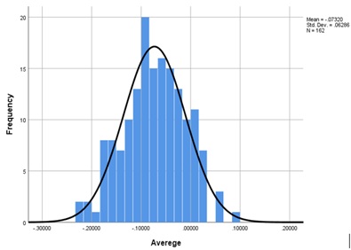Figure 4: Histogram plot for assessing the normality of the fourth coordinate data (outskirts of the city of Heirah) (Source: Current Research).

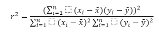
The relationship between the data obtained from the first coordinate (Average1), the third coordinate (Average3), and the fourth coordinate (Average4) was examined (Table 7). Using Pearson correlation coefficients, a weak and positive relationship between the first and fourth coordinates was observed (r = 0.206, p = 0.05 < 0.05 = α), indicating a significant association. Additionally, a moderate and positive relationship was found between the third and fourth coordinates (r = 0.229, p = 0.01 < 0.05 = α). However, there was no significant correlation between the first and third coordinates, showing a very weak and negative relationship (r = -0.035, p = 0.762 > 0.05 = α). These findings indicate that the fourth coordinate is correlated with the other two variables (first and third coordinates), while the first and third coordinates are not correlated with each other. 

According to the obtained results (Table 7), the calculations showed that the data obtained from the fourth coordinate can be explained by 4.2% (r² = 0.206² = 0.042) using the data from the first coordinate and 5.2% (r² = 0.229² = 0.052) using the data from the third coordinate. 

Furthermore, the relationship between the ranked data obtained for the first, second, and third coordinates with the fourth coordinate was examined (Table 8). The reason for analyzing the data in ranked form was due to the non-normality of the data for the second coordinate. Therefore, by transforming the data into their ranks, the possibility of using non-parametric tests was facilitated. 

Correlations

Table 7: Calculation of the coefficient of determination for normality based on Pearson correlation coefficients in an 11-year period (Source: Present study) 

*. Correlation is significant at the 0.05 level (2-tailed). **. Correlation is significant at the 0.01 level (2-tailed). 

Using Spearman correlation coefficients, it was shown that there is a moderate and positive relationship between the ranks of the third and fourth coordinates (ρ = 0.242, p = 0.02 < 0.05 = α). However, the weak and positive relationship between the ranks of the first and fourth coordinates (ρ = 0.189, p = 0.055 > 0.05 = α) and the weak and negative relationship between the ranks of the second and fourth coordinates (ρ = -0.083, p = 0.360 > 0.05 = α) were not significant. These findings indicate that only the rank of the third coordinate is correlated with the fourth coordinate, while the other two variables are not correlated with it. 

Based on the correlation coefficients obtained from the Spearman test (Table 8), it is evident that the coefficient of determination for the fourth coordinate is explained by only 0.7% (r² = -0.083² = 0.007) by the second coordinate and by 3.6% (r² = 0.189² = 0.036) and 5.9% (r² = 0.242² = 0.059) by the first and third coordinates, respectively. 

Correlations 

Table 8: Calculation of the coefficient of determination for ranked data based on Spearman correlation coefficients in an 11-year period (Source: Current Research) 

Based on the output of the Pearson correlation test on the data for the months of August (Table 9), it can be stated that the correlation coefficient between the first and third coordinates is 0.520 (r = 0.520). This indicates a weak to moderate positive linear relationship between these two variables. Additionally, the probability value for this relationship is 0.022, which is smaller than the significance level of 0.05 (p-value = 0.022 > 0.05 = α). In other words, the relationship between these two variables is significant, and the null hypothesis (no relationship) is rejected. It can be said that changes in the first coordinate have led to changes in the third coordinate. Furthermore, there is also a positive linear relationship (weak to moderate) between the Pearson correlation coefficients of water level between the first and fourth coordinates, with a value of 0.445 (r = 0.445). The probability value for this relationship is 0.049, which is smaller than the significance level of 0.05 (p-value = 0.049 > 0.05 = α). Therefore, the relationship between these two variables is also significant, and the null hypothesis is rejected. Thus, changes in water level in the first coordinate result in changes in water level in the fourth coordinate. 

Considering the Pearson correlation coefficients between the months of August for the data related to the first and third coordinates (Table 9), the coefficient of determination is found to be 0.270 (r² = 0.520² = 0.270). This indicates that 27% of the variation in water level in the third coordinate can be explained by the variation in water level in the first coordinate. The coefficient of determination between the first and fourth coordinates was also calculated and found to be 0.198 (r² = 0.445² = 0.198). This means that 19.8% of the variation in water level in the fourth coordinate can be explained by the variation in water level in the first coordinate. 

Correlations

Table 9: Calculation of the coefficient of determination for normal data based on Pearson correlation coefficients for the month of August (Source: Current Study) 

*. Correlation is significant at the 0.05 level (2-tailed). 

The Spearman correlation method (Table 10) was used to examine the correlation coefficients of the August data related to the second coordinates. The reason for using this method was the non-normality of the data in this section. Therefore, nonparametric tests were employed. Based on the results, it can be concluded that there is a positive and significant relationship between the data of the first and third coordinates (Rho = 0.528, Sig = 0.020). Additionally, the relationship between the data obtained from the third and fourth coordinates is positive and significant (Rho = 0.474, Sig = 0.040). However, the relationship between other variable pairs is not significant (Sig > 0.05). This means that the null hypothesis cannot be rejected. 

In the calculation of the coefficient of determination for the August data using the Spearman correlation coefficients (Table 10), the data obtained from the fourth coordinate were explained by 18% (r² = 0.424² = 0.018) through the first coordinate, by 0.2% (r² = 0.047² = 0.002) through the second coordinate, and by 22.5% (r² = 0.474² = 0.225) through the third coordinate. 

Correlations 

Table 10: Calculation of the coefficient of determination for rank data based on Spearman correlation coefficients for the month of August (Source: Current Study) 

*. Correlation is significant at the 0.05 level (2-tailed).

The relationship between the water level of the Euphrates River at various points in three countries, Turkey, Syria, and Iraq, was studied. Satellite imagery data obtained from four points using the NDWI (Normalized Difference Water Index) index and satellite monitoring were examined to assess the dynamics of the river's water level and determine how it is influenced by upstream conditions within the watershed. Therefore, four coastal points within the Euphrates River watershed with a radius of 140 meters were selected. The necessary data for this study were obtained from 546 Landsat 8 OLI/TIRS satellite images covering the period from 2013 to 2022. Suitable statistical methods were employed in the data analysis process to investigate the normality, correlation, and significance of the data (Table 1). 

In the Shapiro-Wilk and Kolmogorov-Smirnov tests, the null hypothesis (H0) is defined as the assumption that the data follow a normal distribution, indicated by a p-value greater than 0.05 (H0: p-value>α=0.05). Conversely, the alternative hypothesis (H1) is defined as the assumption that the data do not follow a normal distribution if the p-value is less than 0.05, denoted as H1: p-value<α=0.05. Accordingly, if the data is found to be significant, parametric tests are used, while non-parametric tests are employed if the data is found to be non-significant. 

The significance of the first coordinate data (p-value=0.200), the third coordinate data (p-value = 0.200), and the fourth coordinate data (p-value=0.200) was investigated and confirmed (Tables 2, 5, and 6) (Figures 1, 3, and 4). The reason for the non-significance of the second coordinate data was that the probability value for this data segment was 0.018 (p-value = 0.018) (Tables 3 and 4) (Figure 2). 

The relationship between the water level at the study points was examined using the Pearson correlation test. Since this test is a parametric test used to measure the linear relationship between two quantitative variables, the data obtained for the first, third, and fourth coordinates were evaluated using this test. The output of this test includes a table of correlation coefficients and the hypothesis test. In the correlation coefficients table, the values of r and Sig are observed for each variable pair. The value of r represents the strength and direction of the relationship between the two variables, ranging from -1 to +1. A value of r close to -1 or +1 indicates a stronger relationship. The sign of r indicates the direction of the relationship, where a negative r represents an inverse relationship and a positive r represents a direct relationship. Sig represents the probability value (p-value) of the hypothesis test. If Sig is smaller than the significance level (α=0.05), it indicates that the relationship between the two variables is significant. 

In the Pearson correlation test, for normally distributed data, the null hypothesis assumes that there is no significant Linear relationship between the water levels of the two coordinates, and it is defined as H0: ρ≠0. On the other hand, the alternative hypothesis is defined as H1: ρ≠0, indicating that there is a significant linear relationship between the water levels of the two coordinates. 

Based on the Pearson correlation coefficients for the 11-year data of the first, third, and fourth variables (Table 7), it was determined that there is a weak but positive relationship between the data of the first and fourth coordinates (r=0.206, p = 0.05 < 0.05=α), confirming the null hypothesis. Similarly, a moderate and positive relationship is observed between the data of the third and fourth coordinates, supporting the null hypothesis (r=0.229, p=0.01 < 0.05=α). The lack of significance in the relationship between the data of the first and third coordinates, despite their weak and negative relationship, indicates the rejection of the null hypothesis, and the alternative hypothesis should be considered valid (r=-0.035, p=0.762>0.05=α). 

Based on the Spearman correlation coefficients (Table 8), it can be concluded that there is a moderate and positive relationship between the ranks of the data of the third and fourth coordinates (ρ=0.242, p=0.02<0.05=α), which supports the null hypothesis. However, the weak and positive relationship between the ranks of the data of the first and fourth coordinates (ρ=0.189, p=0.055>0.05=α), and the weak and negative relationship between the ranks of the data of the second and fourth coordinates (ρ=-0.083, p=0.360>0.05=α) are not significant, indicating the rejection of the null hypothesis and the confirmation of the alternative hypothesis. 

The analysis of data related to the month of August using the Pearson correlation test (Table 9) revealed a correlation coefficient of 0.520 between the data of the first and third coordinates (r=0.520). This indicates the presence of a weak to moderate linear, positive relationship between these two variables. Furthermore, the obtained p-value for this relationship was 0.022, which is smaller than the significance level of the test (p-value=0.022>0.05=α). Therefore, the significance of the relationship between these two variables was confirmed, and the null hypothesis (lack of relationship) was rejected. Additionally, the correlation coefficient between the data of the first and fourth coordinates also indicates a weak to moderate linear, positive relationship (r=0.445). Due to the p-value being smaller than the significance level (p-value=0.049>α=0.05), the significance of the relationship between these two variables was also confirmed, and the null hypothesis was rejected. Hence, based on the obtained results, it can be concluded that changes in the first coordinate will lead to changes in the water level fluctuation in the third and fourth coordinates.

In the Spearman correlation coefficient table, the values of Rho and Sig (2-tailed) are observed for each pair of variables. Rho indicates the strength and direction of the relationship between the two variables. Rho takes values between -1 and +1. The closer Rho is to -1 or +1, the stronger the relationship indicates. The sign of Rho indicates the direction of the relationship. A negative Rho indicates an inverse relationship, while a positive Rho indicates a direct relationship. Sig (2-tailed) represents the p-value of the null hypothesis test. If Sig (2-tailed) is smaller than your chosen significance level (α=0.05), the null hypothesis can be rejected, and it can be concluded that the relationship between the two variables is significant. 

Due to the non-normality of the data for the second set of coordinates (Tables 3 and 4 and Figure 2), non-parametric statistical tests (Spearman correlation) were used to analyze them for the month of August (Table 10). The results indicate a positive and significant relationship between the data of the first and third coordinates (Rho=0.528, Sig=0.020), rejecting the null hypothesis. Additionally, the null hypothesis can be rejected based on the relationship between the obtained data from the third and fourth coordinates, which were positive and significant (Rho=0.474, Sig=0.040). However, the relationship between the other pairs of variables is not significant (Sig>0.05), and the null hypothesis cannot be rejected for them, suggesting that their relationship is random. 

To determine the magnitude of these effects, the coefficient of determination needs to be calculated for the data. This will help determine the percentage of variation in the river water flow in the fourth coordinate (near the outskirts of the city) that can be attributed to the first and third coordinates separately, during the 11-year period and specifically in the month of August. 

The coefficient of determination (r²) was used to examine the magnitude of the ability to explain variations in one quantitative variable by another quantitative variable. The coefficient of determination ranges between 0 and 1. A value closer to 1 indicates that a larger proportion of the variation in one variable can be explained by the variation in the other variable.

R: represents the Pearson correlation coefficient.

r²: represents the coefficient of determination

n: represents the number of observations.

Xi: represents the value of variable x in the observation.

x: represents the mean of variable x.

Yi: represents the value of variable y in the observation.

y: represents the mean of variable y.

Furthermore, using the following formulas, the coefficient of determination can be expressed as the percentage of variance explained. In this formula, R2 represents the squared rank correlation coefficient (Spearman's correlation), and represents the Spearman's correlation coefficient.

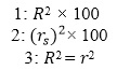
Using the coefficient of determination and considering the results obtained from the analysis of the 11-year data interval using Pearson's test, it can be explained that the fourth coordinate data is explained by the first coordinate data by 4.2% (r²=0.206²=0.042) and by the third coordinate data by 5.2% (r²=0.229²=0.052). However, based on the correlation coefficients obtained from the Spearman's test (Table 8), it was determined that the coefficient of determination for the fourth coordinate data explained by the second coordinate data is only 0.7% (r²= -0.083²=0.007), and by the first and third coordinate data, it is explained by 3.6% (r²=0.189²=0.036) and 5.9% (r²=0.242²=0.059) respectively.

Based on the Pearson correlation coefficients between the months of August for the data corresponding to the first and third coordinates (Table 9), the coefficient of determination is equal to 0.270 (r^2=0.520²=0.270). This means that 27% of the variation in water level in the third coordinate is explained by the variation in water level in the first coordinate. The coefficient of determination between the first and fourth coordinates was also calculated and its value was 0.198 (r² =0.445²=0.198). This means that 19.8% of the variation in water level in the fourth coordinate is explained by the variation in water level in the first coordinate. In the calculation of the coefficient of determination for the August months using Spearman correlation coefficients (Table 10), the obtained data from the fourth coordinate in relation to the first coordinate were explained by 18% (r²=0.424²=0.018), while by the data from the second and third coordinates, they were explained by 0.2% (r²=0.047²=0.002) and 22.5% (r²=0.474²=0.225), respectively.

Based on the findings and results of the Pearson correlation test, as well as the findings of the Spearman correlation test, it can be inferred that over an 11-year period (2013 to 2022), the first and third points individually have an effect on the water flow at the fourth point. Considering that the third point in this study represents the coastal coordinates of Lake Habaniyah, formed behind the Al-Ramadi dam, and that a significant number of dams and barriers have been constructed upstream on the Euphrates River, it is expected that the behavior of this structure would not be different and it would have a similar impact as the upstream structures on the water flow of the Euphrates. Water storage, water diversion, water transfer, and excessive water usage upstream of the Euphrates have shown their influence downstream, specifically at the fourth coordinate. The correlation between the data of the fourth coordinate with the first and third coordinates supports this claim. 

In summary of the results of the Pearson and Spearman correlation tests for the August data, it was observed that the water level at the third coordinate is influenced by the water level at the first coordinate. Additionally, the water level at the fourth coordinate is also influenced by the first point. This means that as the values of the data in the first coordinates increase, the values of the data in the third coordinates will also increase, and higher values in the data of the third coordinates will correspond to higher values in the fourth coordinates. 

In general, it can be stated that the data corresponding to the fourth coordinates are influenced by 3.6% to 4.2% by the data of the first coordinates, and 5.2% to 5.9% by the data of the third coordinates. The findings for the August months also indicate that the fourth coordinates are influenced by 18% to 19.8% by the first coordinates and 22.5% by the third coordinates. Furthermore, the water level at the third coordinates is also influenced by 27% by the first coordinates in the August months. 

The results of data analysis in this study have shown that the water level of the Euphrates River in the outskirts of Lake Hira (Point 4) is directly related to the water level in upstream points. This finding is consistent with the aim of our research, which was to investigate the relationship between water levels at different points of the river. Based on the correlation coefficients and statistical significance, it can be concluded that variations in water level at upstream points have led to changes in the water level at Point 4. 

This research is valuable both scientifically and practically. From a scientific perspective, it introduces a new and suitable method for studying the dynamics of river water levels using satellite data. The advantages of this method include higher accuracy in determining river water levels using the NDWI index, applicability in remote areas, lower cost, and faster data collection. In terms of practical implications, this research can contribute to water resource management. By having precise information about river water levels, water consumption can be optimized and its wastage can be reduced. Additionally, satellite monitoring of river water levels can help predict and prevent hazards caused by droughts or floods, and enhance understanding of sustainable management of freshwater resources. 

This research, like other studies, also had limitations and challenges. These included reliance on high-quality and accurate satellite images, incorrect representation of water levels in the presence of clouds/dust, the inadequacy of the NDWI index for shallow rivers with non-transparent colors, and so on. To overcome these limitations and improve the research, it is suggested to use satellite images with higher resolution and frequency, and to employ optimized methods for image processing to correct colors or eliminate errors. Furthermore, the use of alternative indices for determining river water levels is also recommended. 

Ultimately, this research represents a significant step towards better understanding of river water levels using satellite data and can provide a suitable foundation for future studies.

 I appreciate the efforts of my selfless family and dear friends.

No financial assistance was received for this research, and all expenses were covered by the author.

 The author declares that there is no conflict of interest.

 F.R. is the idea generator, information collector, author, and editor have read the article and agree to its publication.

 It is hereby announced that the data used in this research is freely and publicly available. The link to access the data is: https://zenodo.org/badge/DOI/10.5281/zenodo.8118563.svg.

1. Donchyts G, Winsemius H, Baart F, Dahm R, Schellekens J. et.al (2022) High-resolution surface water dynamics in Earth's small and medium-sized Scientific reports.
2. Moore AMT, Hillman GC, Legge AJ (2009) Village on the Euphrates: from foraging to farming at Abu Hureyra. Oxford University Press.
3. Coad BW (1996) Zoogeography of the fishes of the Tigris-Euphrates Zoology in the Middle East.13: 51-70.
4. Division GBNI (1994) Iraq and the Persian 203-205 (U.K: Distributed in the UK by Marston Book Services New York : Distributed in the US by Columbia University Press).
5. Thomason AK (2001) Representations of the North Syrian Landscape in Neo-Assyrian Art. Bulletin of the American School of Oriental 323: 63-96.
6. Altinbilek D (2002) the role of dams in Water Science and Technology. 45: 169-180.
7. Isaev V, Mikhailova M (2009) the hydrography, evolution, and hydrological regime of the mouth area of the Shatt al-Arab River. Water Resources.36: 380-395.
8. Iraqi Ministries of Environment, R. a. M. a. P. W. Volume I (2006) Overview of Present Conditions and Current Use of the Water in the Marshlands Area/Book 1: Water Resources.
9. Salim MA (2006) MASTER_PLAN_FOR_INTEGRATED_WATER_RESOURCES - 0 (Main Report).
10. Jones C, Sultan M, Yan E, Milewski A, Hussein Hussein MA, al (2008) Hydrologic impacts of engineering projects on the Tigris–Euphrates system and its marshlands. Journal of Hydrology.353: 59-75.
11. Rateb A, Scanlon BR, Kuo C-Y (2021) Multi-decadal assessment of water budget and hydrological extremes in the Tigris-Euphrates Basin using satellites, modeling, and in-situ data. Science of the Total Environment.766: 144337.
12. Al-Ansari N (2013) Management of water resources in Iraq: perspectives and prognoses. Engineering.5: 667-684.
13. Issa IE, Al-Ansari N, Sherwany G, Knutsson S (2014) Expected Future of Water resources within Tigris-Euphrates Rivers basin, Journal of Water Resource and Protection.6: 421-432.
14. Altinbilek D (2004) Development and management of the Euphrates–Tigris International Journal of Water Resources Development.20: 15-33.
15. Adamo N, Al-Ansari N, Sissakian VK (2020) Global Climate Change Impacts on Tigris-Euphrates Rivers Basins. Journal of Earth Sciences and Geotechnical Engineering.10: 49-98.
16. Frenken K (2009) Irrigation in the Middle East Region in AQUASTAT Survey 2008.
17. Kolars JF, William A (1991) the Euphrates River and the Southeast Anatolia Development
18. Jongerden JP (2010) Dams and Politics in Turkey: Utilizing Water, Developing Middle East Policy.17:137-143.
19. Rahman MM, Alam K, Velayutham E (2021) Is industrial pollution detrimental to public health? Evidence from the world's most industrialised BMC Public Health.21:1175.
20. Mulligan M, van Soesbergen A, Sáenz L (2020) GOODD, a global dataset of more than 38,000 georeferenced Scientific Data.7:31.
21. Jamous B (2009) Nouveaux Aménagements Hydrauliques sur le Moyen Euphrate Syrienne. Appel à Projets Archéologiques d'Urgence. Studia
22. Elhadj E (2008) Dry Aquifers in Arab Countries and the Looming Food Middle East Review of International Affairs.
23. Mutin G (2003) Le Tigre et l'Euphrate de la VertigO.
24. Kliot N (1994) Water Resources and Conflict in the Middle Routledge.p: 326.
25. Scheumann W (1998) in Water in the Middle East: Potential for Conflicts and Prospects for Cooperation (eds Waltina Scheumann & Manuel Schiffler).113-135.
26. Daoudy M (2005) Le Partage des Eaux entre la Syrie, l'Irak et la Négociation, Sécurité et Asymétrie des Pouvoirs. CNRS Editions.p: 269.
27. Hillel D (1994) Rivers of Eden: the Struggle for Water and the Quest for Peace in the Middle Oxford University Press.
28. Abdel-Samad M, Khoury A (2006) Water Scarcity In The Middle East balancing Conflict, Development, And Survival In Turkey, Syria And Journal of Peacebuilding & Development.3: 63-74.
29. Dohrmann M, Hatem R (2014) The Impact of Hydro-Politics on the Relations of Turkey, Iraq, and Middle East Journal.68: 567-583.
30. Warner J (2012) the struggle over Turkey’s Ilisu Dam: domestic and international security linkages. International Environmental Agreements: Politics, Law and Economics.12: 231-250.
31. Kibaroglu A, Scheumann W (2013) Evolution of transboundary politics in the Euphrates–Tigris river system: new perspectives and political Global Governance: A Review of Multilateralism and International Organizations.19: 297-305.
32. Kramer A, Kibaroglu A, Scheumann W (2011) Turkey's Water Policy.Springer Science & Business Media.
33. Abdelmohsen K, Sultan M, Ahmed M, Save H, Elkaliouby B, et al (2019) Response of deep aquifers to climate variability. Science of The Total Environment.677: 530-544.
34. Rodell M, Famiglietti JS, Wiese DN, Reager JT, Beaudoing HK al (2018) Emerging trends in global freshwater availability. Nature. 557: 651-659.
35. Voss KA, James S. Famiglietti, Lo M, de Linage C, et. al (2013) Groundwater depletion in the Middle East from GRACE with implications for transboundary water management in the Tigris-Euphrates-Western Iran region. Water Resources Research.49: 904-914.
36. Chang LL, Yuan R, Gupta HV, Winter CL, Niu GY (2020) Why Is the Terrestrial Water Storage in Dryland Regions Declining? A Perspective Based on Gravity Recovery and Climate Experiment Satellite Observations and Noah Land Surface Model With Multiparameterization Schemes Model Water Resources Research.
37. Kareem HH, Alkatib AA (2022) Future short-term estimation of flowrate of the Euphrates river catchment located in Al-Najaf Governorate, Iraq through using weather data and statistical downscaling model.12: 129-141.
38. Abdelmohsen K, Sultan M, Save H, Abotalib AZ, Yan E, et. al (2022) Buffering the impacts of extreme climate variability in the highly engineered Tigris Euphrates river Scientific Reports.12: 4178.
39. Sharma A, Wasko C, Lettenmaier DP (2018) If Precipitation Extremes Are Increasing, Why Aren't Floods? Water Resources 54: 8545-8551.
40. Dai A, Rasmussen RM, Liu C, Ikeda K, Prein AF (2020) A new mechanism for warm-season precipitation response to globalwarming based on convection-permitting simulations. Climate Dynamics.55: 1-26.
41. Dai A (2021) Hydroclimatic trends during 1950–2018 over global Climate Dynamics.56: 4027-4049.
42. Papalexiou SM, Montanari A (2019) Global and Regional Increase of Precipitation Extremes under Global Water Resources Research.55.
43. Winsemius H, et al (2016) Global drivers of future river flood Nature Climate Change.
44. Hirabayashi Y, Roobavannan M, Koirala S, Konoshima L, Yamazaki D, et.al (2013) Global flood risk under climate Nature Climate Change.3: 816-821.
45. Hirabayashi Y, Kanae S, Emori S, Oki T, Kimoto M (2008) Global projections of changing risks of floods and droughts in a changing Hydrological Sciences Journal.53: 754-772.
46. Forsythe DP (2017) Water Security in the Middle East: Essays in Scientific and Social Cooperation (ed Jean Cahan ( 184-167 ) Anthem Press.
47. Anjarini S (2014) in Al Akhbar.
48. Hasan M, Moody A, Benninger L, Hedlund H (2019) How war, drought, and dam management impact water supply in the Tigris and Euphrates Ambio.48: 264-279.
49. O'Connor JE, Duda JJ, Grant GE (2015) Ecology 1000 dams down and Science.348: 496-497.
50. Gonzalez N (2023) The Reasons and Meaning Behind the Euphrates River Drying Up Edition. ,
51. Rahi KA, Halihan T (2009) Changes in the Salinity of the Euphrates River System in Regional Environmental Change.10: 27-35.
52. Jawad LA (2003) Impact of Environmental Change on the Freshwater Fish Fauna of International Journal of Environmental Studies. 60: 581-593.
53. Mutlak F, Jawad L, Al-Faisal A (2017) Atractosteus spatula (Actinopterygii: Lepisosteiformes: Lepisosteidae): A deliberate aquarium trade introduction incidence in the Shatt al-Arab River, Basrah, Iraq. Acta Ichthyologica et Piscatoria.47: 307-310.
54. Muir J (2009) in BBC News (BBC News, K. London, 2009).
55. Al-Daraji S, Jawad LA, Al-Faisal AJ, Taha Yaseen A (2017) Second appearance of the burrowing goby Trypauchen vagina (Bloch & Schneider, 1801) in the marine waters of Iraq. Cahiers de Biologie Marine.58: 229-232.
56. Brunwasser M (2012) Zeugma After the Archaeology Magazine.
57. Abdul-Amir SJ (1988) Archaeological Survey of Ancient Settlements and Irrigation Systems in the Middle Euphrates Region of Mesopotamia PHD thesis, University of Chicago.
58. Solano-Villarreal E, et al (2019) Malaria risk assessment and mapping using satellite imagery and boosted regression trees in the Peruvian Scientific Reports.9:1517.
59. Rajendran S, Sadooni FN, Al-Saad Al-Kuwari H, Oleg A, Govil H, et.al (2021) Monitoring oil spill in Norilsk, Russia using satellite Scientific Reports.11:3817.
60. Mateo-Garcia G, Veitch-Michaelis J, Smith L, Vlad Oprea S, Schumann, G, et. al (2021) towards global flood mapping onboard low cost satellites with machine Scientific Reports.11: 7249.
61. McFeeters SK (1996) the use of the Normalized Difference Water Index (NDWI) in the delineation of open water International Journal of Remote Sensing.17: 1425-1432.
62. Xu H (2006) Modification of Normalized Difference Water Index (NDWI) to Enhance Open Water Features in Remotely Sensed International Journal of Remote Sensing.27: 3025-3033.
63. Hui C, Guo Y, Li H, Gao C, Yi J (2022) Detection of environmental pollutant cadmium in water using a visual bacterial Scientific Reports.12: 6898.
64. Chen W, Wang D, Huang Y, Chen Lid, Zhang L, et. al (2017) Monitoring and analysis of coastal reclamation from 1995–2015 in Tianjin Binhai New Area, Scientific Reports.7: 3850.
65. Figliomeni FG, Guastaferro F , Parente C, Vallario A (2023) A Proposal for Automatic Coastline Extraction from Landsat 8 OLI Images Combining Modified Optimum Index Factor (MOIF) and K-Means. Remote Sensing 15: 3181.
66. Almar R, Boucharel J, Graffin M, Ondoa Abessolo G, Thoumyre G, et.al (2023) Influence of El Niño on the variability of global shoreline position. Nature Communications.14: 3133.