Assessing Trend Changes in Functional and Structural Characteristics: Combining Principal Components Methods and Functional Data Analysis
*Corresponding Author(s):
Johannes LedolterDepartment Of Business Analytics And Department Of Statistics And Actuarial Science, University Of Iowa, Iowa City, IA 52242, United States
Email:johannes-ledolter@uiowa.edu
Abstract
We illustrate the technique - functional data analysis to create a complete data matrix and principal components analysis to determine the most important features for classification - on the average thickness of the retinal nerve fiber layer that come from two groups of patients.
Keywords
MATHEMATICS SUBJECT CLASSIFICATION
INTRODUCTION
In reference [1] we discuss how to 1) Best analyze multiple short time series of functional and structural characteristics collected on different groups of subjects and (2) Classify subjects on the basis of their time progression. These methods help us assess the progression of measurements taken over time, such as the visual acuity of normal and glaucoma subjects (measured by either a visual field test or by Optical Coherence Tomography (OCT) measurements on the optic nerve) or the weight gains of children on different diets. Common difficulties with the analysis of such data are the relatively short length of each time series and the fact that measurements are taken at time periods that vary across subjects.
In reference [1] we consider random effects (repeated measurement) time-trend models of the form Yt = α+βTimet+noiset and discuss how such models can be estimated on time series observations from multiple subjects of several groups. Model results can be used to test whether or not the average slopes (or the variances of slopes across subjects) of different groups are the same.
We also discuss how subject-specific least squares estimates of intercept and slope in the trend model can be used to classify subjects into one of several groups. Such classification can be carried out with Fisher’s linear or quadratic discriminant functions [2,3], or with a non-parametric support vector machine algorithm [4,5]. However there are shortcomings with this approach as it assumes that the investigator has already decided on the intercept and slope as the relevant summary statistics for a subject’s time progression. An alternative strategy that is discussed in this paper determines the relevant summary features through principal components analysis and classifies the subjects on their scores that result from the most important principal components. Since observations on the subjects are usually not taken at the same time, we first need to transform the irregularly-spaced data into a complete matrix of observations with rows representing subjects and columns representing time. We use functional data analysis techniques to construct this data matrix. We discuss the methods in Section 2, and illustrate the analysis in Section 3 on OCT data collected on normal and glaucoma subjects.
A NONPARAMETRIC APPROACH FOR CLASSIFYING TIME SERIES DATA
Reducing the dimensions of a time series through principal components and classifying subjects on their implied principal components scores
The goal is to classify subjects on their time progression. Imagine the case when we have observations on m subjects taken at the very same T time points. If T is large (say observations at monthly intervals over a period of 10 years, and hence T = 120), the classification takes place in a very high-dimensional (120-dimensional) feature space. A way to simplify the problem is to reduce the T observations to a smaller number of subject-specific summary features and classify the subjects on their summary features. Summary features can be pre-selected, such as the intercept and the slope of the trend regression considered in reference [1]. Another approach is to treat the measurements at the T time periods as features, determine the principal components, hence reducing the dimensionality of the classification by classifying the subjects on their scores that are implied by the most important principal components. The (length-standardized) weights of the first principal component represent the coefficients in the linear combination of the T measurements that has the largest variance. The weights of the second principal component determine the linear combination that has the largest variance among all linear combinations whose weights are orthogonal to the weights of the first principal component; and so on. The weights are also referred to as the principal component loadings on the features. The mathematics is rather simple and involves the calculation of the largest eigenvalues of the T x T sample covariance matrix (which is estimated from the time series data on the m subjects). The ordered eigen values of the covariance matrix, d1,d2,... represent the variances that are explained by the first, second, … most-important principal components. And the corresponding eigenvectors are the weights (loadings) of the principal components. Note that the rank of the T x T sample covariance matrix can never be larger than min(m-1,T). For m≤T, the sample covariance matrix is singular and at least T-m+1 of its eigenvalues are zero.
We are dealing with the time progression of multiple subjects when measurements on all subjects are taken at the same time points. Graphically, the information can be visualized as follows. We start by drawing the mean curve, which we obtain by averaging the responses across the m subjects and at each of the T time points and by connecting the successive averages. A multiple of the first principal component weights (with multiple 2√d1, where d1 is the variance explained by the first principal component) is added to and subtracted from the mean curve, resulting in two (a lower and an upper) PCA weight curves for the first principal component. Assume, for illustration, that there is a considerable subject effect to the time progression and suppose that the time progression curve shifts up or down depending on the subject. In this case the T x T correlation matrix has large positive correlations at all off-diagonal elements (as being above average at a particular time point means also being above average at other time points). The weights of the largest principal component in this case are all equal, implying that the first principal component score for a subject is the average of its T observations. For this particular illustration the resulting graph of the (lower and upper) first PCA weight curves reflects a band of equal width around the mean curve, with bands far from the mean curve if the principal component explains much of the total variance. In other words, a graph with such “banded” PCA weight curves suggests that subject levels (averages) carry useful information for classification. [Mathematically, for a T x T matrix of all ones, the largest eigenvector is T while all other eigenvectors are 0, and the eigenvector corresponding to the largest eigenvector is proportional to the vector of all ones].
As a second illustration, assume that the time progression curves of subjects are linear, but with different subject-specific slopes. In this particular case the weights of the (first) principal component are linear in time with mean zero. Adding and subtracting 2√d1 multiples of the principal component weights from the mean curve results in two crossing lines, and the closeness of the lower and upper PCA weight curves from the average curve reflects how much variability is explained by the principal component. Because of the linearity of the weights, a subject’s principal component score assesses the magnitude of its slope (but is unaffected by the level).“Crossing” PCA weight curves are an indication that there is useful information in the slopes. The usefulness of the corresponding PCA scores for classification purposes will be small if the lower and upper PCA weight curves are close to the average curve. [Mathematically, consider the time trend Yt = c+β(t-t?), for t=1,2,...,n and let the slope β vary across subjects with Var(β)=σ2β. In this case the T x T covariance matrix of the observations has rank 1 and the eigenvector corresponding to the one positive (largest) eigenvector is proportional to (t-t?), a linear function of time with mean zero. The resulting PCA score measures a subject’s slope, but is not affected by the subject’s level].
PCA weight curves provide information on the important features of multiple time series. For example, two major principal components with “banded” and “crossing” PCA weight curves indicate that the levels and the slopes of the time progression functions carry useful information for classification. The variances explained by these two principal components (and the closeness of the PCA weight functions from the average response curve) express how well a subject’s level and slope represent the time progression. Often only scores from the first or the first two principal components are needed for classification, but there could be situations where more than two principal components are needed. Furthermore, the scores resulting from the most important principal components need not be the subject’s mean and the slope.
In paper [1] we characterize the time-progression of each subject with a parametric (linear) model. We compare and classify subjects on the estimated summary statistics from that model which – for the linear model – are the intercept and the slope of the fitted trend regression line. The approach in this note is non-parametric and more general as it uses the scores from the most important principal components; the resulting scores don’t necessarily have to be the intercept (average) and the slope, and there can be more than two scores.
The functional data analysis approach for data collected at different time periods
Even quite complicated response functions of time can be approximated by linear combinations of either Fourier or spline basis functions. A rich basis with many basis functions allows for a very general representation. Ordinary least-squares estimates are available if the number of basis functions is less (or equal) than the number of observations. However, with a rich class of basis functions and its many estimates, the fitted response function will be rather noisy. A smoother response function results when introducing a penalty for the roughness of the fitted function. The square of the second derivative of a function at a fixed argument expresses the deviation from linearity as the second derivative disappears for a linear function. Hence, a useful measure of roughness of a function is the integrated squared second derivative of the function, with integration extending over the function’s range. Penalized regression determines the estimates by minimizing the sum of the error sum of squares and a multiple of the roughness of the function; the multiple is referred to as the smoothing parameter or the penalty λ. By increasing the penalty, the fitted response function reduces to the linear least squares line. Cross-validation techniques determine the appropriate penalty λ that needs to be imposed, letting the data themselves dictate the smoothness of the response function. Introduction of a penalty into the estimation has yet another advantage because it allows us to consider more basis functions than the number of available observations; with least squares estimation alone, this would not be possible. The general cross-validation measure developed [9], standardizes the error sum of squares by the (square of the) effective degrees of freedom of the fit (which depend on the smoothing parameter and the hat regression matrix). Software is readily available to obtain the smoothing parameter that minimizes the cross-validation measure; we use the fda package of the R Statistical Software [10].
A penalized regression on B-splines of degree g = 2 with knots at all distinct time periods across all subjects is used to estimate the response curve for each subject. A penalty for the roughness of the fitted function is introduced, and the optimal smoothing coefficient is obtained by minimizing the average of the general cross-validation scores across all subjects. This allows the data to determine the appropriate functional form of the time progression and does not limit the analyst to a specific functional form such as the linear time-trend model considered previously in reference [1]. The response for each of the m subjects is then evaluated at the T* = 50 equally-spaced time periods covering the interval from the smallest to the largest time point. The function pca.fd from the fda package is used to carry out the principal components analysis on the regular array-type data structure for the m subjects and T* = 50 periods, display the PCA weight curves discussed in the previous section, and calculate the implied principal components scores. The mean response and the PCA weight functions can also be smoothed for better interpretability. Subjects are then classified on their implied principal components scores, using either linear or quadratic discriminant functions.
EXAMPLE
We find that we need no more than two principal components to describe the variability in the time response function. The first principal component alone explains 98.1 (GCL) and 99.0 (RFNL) percent of the total variation. The wide and roughly parallel bands in the PCA curves for the first principal component (left panel) indicate a very large subject effect (Figure 1). The crossing lines for the PCA curves for the second principal component (right panel), with their small deviations from the average trend line, indicate very minor variability in the subjects’ slopes. This fact is confirmed by the small proportions of variability (1.7 percent for GCL and 1 percent for RNFL) that are explained by the second principal components. Scores of the first two principal components are calculated for all subjects, and linear and quadratic discriminant functions are used for classification. Scatter plots of first and second PCA scores are shown in Figure 2. Normal subjects are shown as red dots and glaucoma subjects are shown as blue dots. Subjects that are misclassified by Fisher’s quadratic discriminant function are displayed with an open circle in a color that reflects the incorrect classification. A red dot with a blue circle indicates a normal subject incorrectly classified as coming from the glaucoma group. A blue dot with a red circle indicates a glaucoma patient incorrectly classified as coming from the normal group.
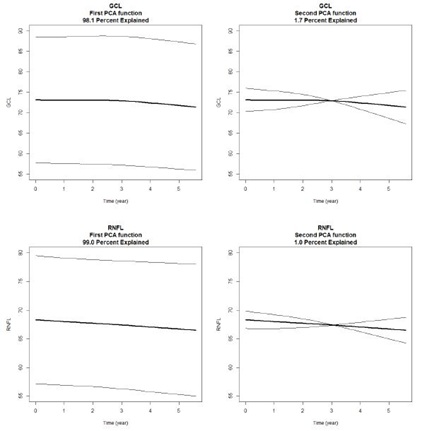 Figure 1: Mean response function (bold) with added first (and second) principal components weights, for GCL (top) and RFNL (bottom). Levels are much more important than slopes for classification.
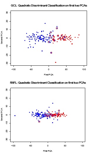 Figure 2: Scatter plots of first and second PCA scores. Normal subjects are shown as red dots and glaucoma subjects are shown as blue dots. Subjects that are misclassified by the quadratic discriminant function are displayed with an open circle in a color that reflects the incorrect classification. A red dot with a blue circle indicates a normal subject incorrectly classified as coming from the glaucoma group. A blue dot with a red circle indicates a glaucoma patient incorrectly classified as coming from the normal group.
Misclassification errors for quadratic discriminant functions are listed in Table 1. The misclassification rates (8.8 percent for GCL and 13.2 for RFNL) are very similar to the misclassification rates we reported in [1], when using least squares estimates of intercepts and slopes. Misclassification errors for quadratic discriminant functions when using the scores of the first principal component alone are only slightly larger; 17/159 = 0.107 for GCL and 25/159 = 0.157 for RFNL. This was expected as the first principal component (which measures the average level of a subject) alone explains about 99 percent of the total variation. The second principal component (which measures the slope) contributes little to the classification. Here we report misclassification rates that are based on the complete data set; results from resampling test-training splits are similar.
|
GCL |
|||
|
Classified as |
|||
|
True Group |
NORMAL |
GLAUCOMA |
|
|
NORMAL |
5 |
14 |
|
|
GLAUCOMA |
10 |
94 |
|
|
Overall misclassification rate: 14/159 = 0.088 |
|||
|
RNFL |
|||
|
Classified as |
|||
|
True Group |
NORMAL |
GLAUCOMA |
|
|
NORMAL |
4 |
96 |
|
|
GLAUCOMA |
15 |
89 |
|
|
Overall misclassification rate: 21/159 = 0.132 |
|||
Table 1: Cross-classification matrix and misclassification rates of quadratic discriminant functions applied to the first two principal components scores, for GCL and RFNL.
CONCLUSION
FUNDING
REFERENCES
- Ledolter J, Kardon RH (2018) Assessing trends in functional and structural characteristics: A survey of statistical methods with an example from ophthalmology. Transl Vis Sci Technol 7: 34.
- Johnson RA, Wichern DW (2012) Applied Multivariate Statistical Analysis (6th Edn). Essex, UK.
- Ledolter J (2013) Data Mining and Business Analytics with R. John Wiley & Sons, New York, USA.
- Boser BE, Guyon IM, Vapnik VN (1992) A training algorithm for optimal margin classifiers. COLT '92 Proceedings of the fifth annual workshop on Computational learning theory Pg no: 144-152.
- Cristianini N, Shawe-Taylor J (2000) An Introduction to Support Vector Machines and other Kernel-based Learning Methods. Cambridge University Press, Cambridge, UK.
- Ramsay JO, Hooker G, Graves S (2009) Functional Data Analysis with R and MATLAB. Springer-Verlag New York, New York, USA.
- Ramsay JO, Silverman BW (2002) Applied Functional Data Analysis: Methods and Case Studies. Springer-Verlag New York, New York, USA.
- Ramsay JO, Silverman BW (2005) Functional Data Analysis. Springer, New York, USA.
- Craven P, Wahba G (1978) Smoothing noisy data with spline functions Estimating the correct degree of smoothing by the method of generalized cross-validation. Numerische Mathematik 31: 377-403.
- Ramsay JO, Wickham H, Graves S, Hooker G (2018) Package ‘fda’.
Citation: Ledolter J (2019) Assessing Trend Changes in Functional and Structural Characteristics: Combining Principal Components Methods and Functional Data Analysis. J Ophthalmic Clin Res 6: 057.
Copyright: © 2019 Johannes Ledolter, et al. This is an open-access article distributed under the terms of the Creative Commons Attribution License, which permits unrestricted use, distribution, and reproduction in any medium, provided the original author and source are credited.