Estimating Ancestry from a Recovered Cranium Using the FORDISC 3.I Computer Program: A Possible Case of Admixture-Case Report

On February 20, 2008, this biological anthropologist presented a paper titled “Admixture and the Growing List of Racial Categories: Clarity or Confusion for Law Enforcement (and the Public)” at the Proceedings of the American Academy of Forensic Sciences 60th Anniversary Scientific Meeting in Washington, DC. The biological anthropologist expressed the general point that in publicizing missing people, law enforcement must be able to use racial categories that are most familiar to the general public to increase the likelihood of finding these missing people and thus bring closure for families [1]. While the goal of bringing closure for families remains sacrosanct, immigration and racial admixture (i.e., interracial ancestry) are blurring the familiar racial categorical lines. 

“Race” is a convenient social tool that law enforcement employs for many practical purposes, an important one being to find people when they go missing. However, the steady increase in biracial or triracial population groups and the constant flow of immigrants to the United States in the past sixty years have complicated the racial picture to the point where it is becoming difficult to fit people into their neat racial categories as depicted on job application forms (Figure 1).

Figure 1: U.S. Census form 2010 showing the growth in racial categories in the past sixty years due to the constant flow of immigrants to the U.S. 

Racial admixture in the United States goes back to the seventeenth century [2]. In the aftermath of the civil rights movement in the late 1960s and 1970s and subsequently enlightened attitudes about race, interracial relationships have steadily increased, accompanied by a parallel increase in the population of biracial children. With the multicultural mix added by immigrants (Figure 1), the US Census Bureau (in coordination with the federal and state governments) has further subdivided racial categories to reflect the growing multiracial mix. For example, relatively new racial categories include Guamanian, Chamorro, Samoan, Laotian, Hmong, Fijian, Tongan, Cambodian, and Pakistani, to name a few [3]. While this attempt to document the reality of the US population’s composition is laudable-because popular categories of race are already biologically a questionable concept-it adds to the already difficult task of the police in finding missing people and pinpointing admixture phenotypically [4-11]. For example, in looking at a photograph, the police might by default lump the Guamanian, Chamorro, Fijian, Tongan, and Pakistani ethnic groups into the familiar categories of Native American, Hispanic, Latino, or Mexican—the categories Hispanic, Latino, and Mexican have their own ambiguity—and lump the Laotian, Hmong, and Cambodian ethnic groups into the Asian category. 

In November 2012, this biological anthropologist collected craniometric data from a cranium found in a wooded area of Newport Township in Luzerne County, Pennsylvania. He processed the measurement data with the FORDISC 3.1 computer program, which indicated admixture, specifically a mixed-race individual.

Case report (PO4-0744558)      

On November 16, 2012, two people searching for cans and bottles in a wooded area off Alden Mountain Road in Newport Township, Luzerne County, Pennsylvania, discovered a partially buried human cranium. Investigators from Pennsylvania State Police Troop P Shickshinny station designated the case as PO4-0744558. The biological anthropologist arrived at the scene within twenty-four hours of the discovery and aided in the search for additional biological and nonbiological materials. Unfortunately, the search was unsuccessful because detectives did not give a clear provenience for the cranium within the 2,125-acre wooded area. A cadaver dog was enlisted in the search to find remains, but nothing was found. A quick visual assessment of the cranium indicated a slightly weathered cranium with no mandible and possible animal gnawing on the frontal, parietal, and occipital bones (Figure 2a-b). The cranium was transferred to the custody of the anthropologist for analysis on November 21, 2012, several days after the county coroner completed his examination (Figure 3).

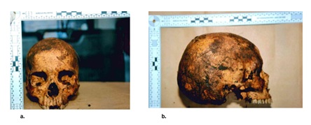Figure 2a-b: The unknown in frontal, profile, and posterior views before (a, b, e) and after cleaning (c, d) [Some of the images are not equal scale].

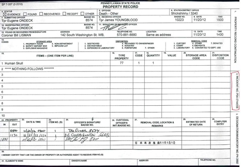Figure 3: Pennsylvania State Police Property Record form with case incident number P04-0744558 and signatures showing chain of custody.

The biological anthropologist gently cleaned the cranium with a soft bristle brush and manicure sticks to remove sediment (very dark brown sediment—7.5YR 2.5/3 on the Munsell scale), small dry leaves, and tiny root structures from the respective foramina of the cranium [12] (Figure 2c–d). He then documented and collected this material (Figure 4). Soil embedded in cranial foramina indicated previous, either natural or unnatural, burial of the remains [13].

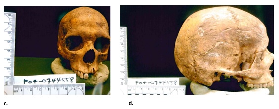Figure 2c-d: The unknown in frontal, profile, and posterior views before (a, b, e) and after cleaning (c, d) [Some of the images are not equal scale].

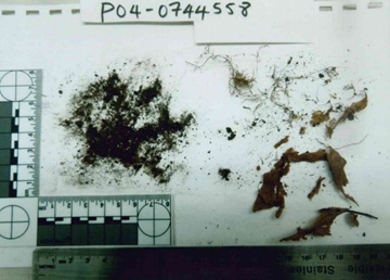Figure 4: Dark brown sediment-7.5YR 2.5/3 on the Munsell scale), small dry leaves, and tiny root structures removed from unknown cranium. 

A detailed visual assessment of the cranium showed the skull was small with moderate brow ridges, sharp orbital rims, a non-projecting mastoid process, and a smooth nuchal region. Additionally, the facial profile was straight, with receding cheek bones and a triangular nasal opening with a narrow nasal root and large nasal spine. Finally, the teeth indicated minimal wear-the incisors were blade-shaped and the third molars not fully erupted (Figure 2e).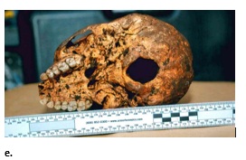Figure 2e: The unknown in frontal, profile, and posterior views before (a, b, e) and after cleaning (c, d) [Some of the images are not equal scale].

Craniometrics 

The biological anthropologist used conventional instruments (i.e., sliding digital calipers and digital and traditional spreading calipers) to collect the metric measurements on the cranium in November 2012 (Figure 5). Craniometrics have proved valuable in assessing large-scale relationships among populations, conducting small-scale analyses among populations, and, in the forensic context, aiding in the identification of unknown skeletal remains [14-16]. In hindsight, the biological anthropologist would have used a MicroScribe digitizer to better capture cranial size and shape, and three-dimensional (3D) osteometric landmark coordinate data as used in his current research [17]. Nevertheless, the craniometric measurements used in this case are described in (Table 1), and the corresponding cranial landmarks are shown in Figure 6a–c. These cranial measurements are found in the FORDISC 3.1 computer program for several comparative reference groups. Specifically, there are fifty-six landmarks (forty-two measurements) in the Forensic Data Bank (FDB) and thirty-nine new measurements (in addition to the fifty-six landmarks) in the William W. Howells Craniometric Data Set. Only cranial measurements in the FDB will be used in this analysis.

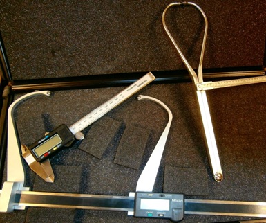 Figure 5: Spreading and sliding digital calipers used in collection of craniometric measurements.

Table 1: Craniometric landmarks used in the FDB in FORDISC 3.1 listed by abbreviation, measurement, and brief description (Adapted from Fleischman and Crowder 2019; Buikstra and Ubelaker 1994).

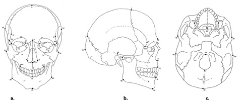 Figure 6a-c: Cranial measuring points in (a) frontal, (b) profile, (c) posterior views. 

(Adapted from Buikstra and Ubelaker 1994).

FORDISC 3.1 generates an unknown cranium’s posterior and typicality probability of membership in each reference group in the database. Posterior probabilities sum to 1 (100 percent) and are based on the unknown cranium’s relative similarities (all Mahalanobis distances [D²]) to all groups [18]. A high posterior probability, which in turn creates a small distance, indicates a greater similarity than to other groups. Typicality probabilities (Typ), in contrast, are the unknown cranium’s probability of membership in each group, based on its absolute similarity. The percentage of correct group allocations-or groups with the typical profile of the unknown’s case—is an indication of how well groups can be separated using the available variables. The word “typical” used above is important because distance probabilities or “typicality probabilities” can be calculated to ascertain whether an individual is typical for a specific group (and not assumed to belong to a respective group, as in posterior probabilities). When the typicality probabilities are uniformly low (i.e., less than 0.01 for each group), the posterior probabilities and classification should be disregarded because classification accuracy is critical in biological evidence for affiliation [19]. An important result is that the D² values will follow a chi-square distribution with a p degree of freedom.

Additionally, FORDISC 3.1 uses canonical variates to display data in graphic form. Canonical variate analysis is most effective in problems where many variables are used to compare differences among and within many reference groups. This analytical technique uses raw data to produce coefficients (or eigenvectors), which are used to obtain new variables called canonical variates that maximize the among-groups variation (eigenvalues) relative to the standardized within-groups variation [20]. The variables (or measurements) are combined into a reduced number of functions to maximize the separation between groups. Such plots provide visual information about which sample means (or centroids) are close to or distant from one another in multivariate space. Moreover, multidimensional data space transforms confidence “intervals” into confidence “spheroids” (or ellipses), which are equidistant with regard to the within-group dispersion. Finally, there are usually several canonical variates independently holding biological information. However, it is the earlier variates that will contain information such as differences in overall shape and size.

Analysis of unknown cranium 

After collecting the craniometric measurements from the cranium, the anthropologist recorded them in the FDB in FORDISC 3.1 (Table 2). The biological anthropologist used all cranial and FORDISC 3.1-calculated measurements (i.e., NAA, PRA, BAA, NBA, BBA, BRA) in the FDB (Table 2). Because there was no clear information on ancestry and sex for this cranium, all female reference groups (i.e., White, Black, Hispanic, American Indian, and Japanese) and all male reference groups (i.e., White, Black, Hispanic, Guatemalan, American Indian, Japanese, Vietnamese, and Chinese) were used in the analysis. The term “American Indian” (as opposed to Native American) is the language used in the FORDISC 3.1 FDB. 

Table 2: Craniometric data collected from cranium and recorded in FDB in FORDISC 3.1∞. 

∞Additional Measurements automatically calculated and only found in FDB in FORDISC 3.1:

NAA: Nasion angle; PRA: Prosthion angle; BAA: Basion angle; NBA: Nasion angle; BBA: Basion Angle; BRA: Bregma Angle 

On the initial computing of measurements, FORDISC 3.1 classified the cranium into the Hispanic female (HF) reference group with a posterior probability of 0.468 (Table 3). The typicality probabilities were 0.136 (Typ F, which is dependent on sample size), 0.093 (Typ Chi, which is not dependent on sample size), and 0.200 (Typ R, where the cranium was ranked twenty-fourth out of thirty individuals within the group). In essence, this cranium is typical of 80 percent of Hispanic females. Additionally, this cranium is within the range of variation of White females with a posterior probability of 0.393. Regardless, the typicality R is higher for the Hispanic female reference group than the White female reference group (0.110). In other words, this unknown cranium fits better into the Hispanic female range of variation than in the White female range. 

Table 3: FORDISC 3.1 classification of unknown cranium in the FDB (all male and female reference groups).

Multigroup Classification of Current Case. 

α Reference groups: HF = Hispanic females; WF = White females; BF = Black females; AF = American Indian females; WM = White males; HM = Hispanic males; BM = Black males; JF = Japanese females; GTM = Guatemalan males; Guatemalan males; JM = Japanese males; CHM = Chinese males; AM = American Indian males; VM = Vietnamese males

BOLD & red: unknown cranium not typical for these groups 

A graph of the results depicted in a 3D canonical space showed this variation (Figure 7). Surprisingly, the unknown cranium, (indicated by the bold “X” in the graph) is closest to the White female reference group’s centroid, but the ellipses of the White and Hispanic reference groups overlap, and the Hispanic group’s centroid is within the ellipse of the White reference group. See Supplement 1 for additional FORDISC 3.1 descriptive data. In this analysis, 61.2 percent of the reference groups in FORDISC 3.1 were classified correctly.

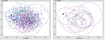Figure 7: FORDISC (FDB) graph classification results all male and female reference groups in canonical space: a) within and between groups scatter; b) without groups scatter. Unknown cranium ‘X’ is close to the centroid of WF reference group. 

The FORDISC 3.1 classification results for this unknown cranium indicate that posterior probabilities are distributed among Hispanics and Whites. This is often associated with mixed-race groups, and Hispanics are culturally and genetically heterogeneous, with European, Native American, and African ancestral populations [21-22]. In admixture genetic analyses research (1991 and 2003) using samples of six autosomal DNA markers from nine Hispanic populations from different regions of the United States, geneticists generated the following admixture coefficients: 82.89 percent European (Pennsylvania); 84.49 percent European (New Jersey); 65.60 percent European (San Antonio); 68.30 percent European (Arizona); 83.40 percent European (Los Angeles); 17.11 percent African (Pennsylvania); 6.38 percent African (New Jersey); 2.50 percent African (Arizona); 9.14 percent Native American (New Jersey); 34.40 percent Native American (San Antonio); and 16.60 percent Native American (Los Angeles) [23-24]. In essence, this cranium could belong to an individual who is of mixed race.

In waiting eleven years to write this case report, the biological anthropologist was hoping for a resolution of this case to compare an actual photograph of the victim (phenotype—social race) to the results that FORDISC 3.1 generated (craniometrics—biological or ancestry). DNA extracted from the cranium in 2013 generated no match on the Combined DNA Index System used by law enforcement. To date, this case has not been resolved.

1. Quintyn C (2008) Admixture and the growing list of racial categories: Clarity or confusion for law enforcement (and the public). Proceedings of the American Academy of Forensic Sciences 60^th Anniversary Scientific Meeting 14: 347.
2. Katarzyna B, Durand EY, Macpherson JM, Reich D, Mountain JL (2015) The genetic ancestry of African Americans, Latinos, and European Americans across the United States. Am J Hum Genet 96: 37-53.
3. https://www.census.gov/programs-surveys/decennial-census/technical documentation/questionnaires.2020_Census.html
4. Brace CL (2005) Race is a four-letter word: The genesis of the concept. New York: Oxford University Press.
5. Graves JL (2004) The race myth: Why we pretend race exists in America. New York: Penguin Books.
6. Cartmill M (1999) The status of the race concept in physical anthropology. Am Anthropol 100: 651-660.
7. Goodman AH, Armelagos GJ (1996) The resurrection of race: The concept of race in physical anthropology in the 1990s. In: Larry T. Reynolds and Leonard Lieberman (eds.). Race and Other Misadventures: Essays in Honor of Ashley Montagu in his Ninetieth Year: 174-186.
8. Gordon CC (1993) Why classify race? In: Claire Gordon (ed.). Race, Ethnicity, and Applied Bioanthropology: 1-6.
9. Gordon CC, Bell NA (1993) Problems of racial and ethnic self-identification and classification. Race, Ethnicity, Applied Bioanthropology 34-47.
10. Sauer NJ (1993) Applied anthropology and the concept of race: A legacy of Linnaeus. In: Claire Gordon (ed.). Race, Ethnicity, and Applied Bioanthropology 79-83.
11. Sauer NJ (1992) Forensic anthropology and the concept of race: If races don’t exist, why are forensic anthropologists so good at identifying them? Soc Sci Med 4: 107-111.
12. Munsell (2000) Soil color charts. New Windsor, New York: GretagMacbeth.
13. Ubelaker DH (1997) Taphonomic applications in forensic anthropology In: William D. Haglund and Marcella H. Sorg (eds.). Forensic Taphonomy: The Postmortem Fate of Human Remains 77-90.
14. Ousley SD, Ashley M (2001) Three-dimensional digitizing of human skulls as an archival procedure. In: Emily Williams (ed.). Human Remains: Conservation, Retrieval, and Analysis: Proceedings of a Conference held in Williamsburg 173-184.
15. Howells WW (1973) Cranial variation in man: A study by multivariate analysis of patterns of difference among recent human populations. Papers of the Peabody Museum of Archaeology and Ethnology 67.
16. Jantz RL (1971) Microevolutionary change in Arikara crania: A multivariate analysis. Am J Phys Anthropol 38: 15-26.
17. Quintyn CB (2022) Questionable affiliation of five curated human crania: Using microscribe 3D digitizer and FORDISC 3.1 computer program to estimate ancestry and sex. J Forensic Res 13: 516-526.
18. Ousley SR, Hollinger E (2009) A forensic analysis of human remains from a historic conflict in North Dakota. In: Dawnie W. Steadman (ed.). Hard Evidence: Case Studies in Forensic Anthropology 91-102.
19. Jantz RL, Stephen DO (2005) Fordisc 3.0: Personal Computer Forensic Discriminant Functions. Knoxville, TN: The University of Tennessee.
20. Albrecht G (1980) Multivariate analysis and the study of form, with special reference to canonical variate analysis. Am Zool 20: 679-693.
21. Chakraborty BM, Fernández-Esquer ME, Chakraborty R (1999) Is being Hispanic a risk factor for non-insulin dependent diabetes mellitus (NIDDM)? Ethn Dis 9: 278-283.
22. Sans M (2000) Admixture studies in Latin America: From the 20th to the 21st century. Hum Biol 72: 155-177.
23. Bertoni B, Budowle B, Sans M, Barton S, Chakraborty (2003) Admixture in Hispanics: Distribution of ancestral population contributions in the continental United States. Hum Biol 75: 1-11.
24. Long JC, Williams RC, McAuley JE Medis R, Partel R, et al. (1991) Genetic variation in Arizona Mexican Americans: Estimation and interpretation of admixture proportions. Am J Phys Anthropol 84: 141-157.