Impact of Background Noise in Mobile Phone Networks on Forensic Voice Comparison
*Corresponding Author(s):
Balamurali BT NairDepartment Of Electrical And Computer Engineering, Forensic And Biometrics Research Group (FaB), The University Of Auckland, Auckland, New Zealand
Tel:+64 93737599,
Email:bbah005@aucklanduni.ac.nz
Abstract
This paper examines the impact of Background Noise (BN) originating at the transmitting end of a mobile phone transmission on the subsequent performance of a forensic voice comparison analysis. The investigation covers the two major mobile phone technologies currently in use globally, namely the Global System for Mobile Communications (GSM) and Code Division Multiple Access (CDMA). It is shown that both networks handle BN in a different way, and for both, BN negatively impacts the accuracy of a FVC analysis. At low levels of BN, this impact is small for both networks. As expected, it increases as the level of BN increases, but surprisingly is worse for CDMA-coded speech, this being attributed to that network’s unique noise suppression process. As far as the precision of a FVC analysis is concerned, interestingly this is shown to improve with increasing BN irrespective of the network origin.
INTRODUCTION
Speech evidence elicited from mobile phone recordings can play an important role in criminal trials. But these recordings are often corrupted by large amounts of Background Noise (BN) picked up by the sending-end microphone during a call. The extent to which this might impact upon the subsequent processing of the speech signal varies from one mobile phone network to another. There are currently two major technologies in the mobile phone arena, namely the Global System for Mobile Communication (GSM) and Code Division Multiple Access (CDMA). These are different in their design and in their ways of handling such noise-corrupted speech. One of the key differences between the GSM and CDMA network is in respect to a process called Noise Suppression (NS), which is only present in the CDMA network.
NS is used in the CDMA network for two purposes: (i) to reduce the BN in each speech frame, and (ii) to improve the subsequent classification of speech frames into voiced, voiceless (often referred to as unvoiced) and silence, this being necessary for the coding process used by this network [1]. Despite the success of NS in reducing noise, it has been reported to remove part of the original speech when the BN levels are high, such as would be the case when a call originates from a moving vehicle [2]. The primary goal of this paper is to investigate the impact of BN in the mobile phone arena on the strength of speech evidence arising from a Forensic Voice Comparison (FVC) analysis. Mobile network operators, when testing the performance of their codecs under various noise conditions, typically use three types of noise: babble noise (i.e., confused sound or perhaps background speech of a group of people talking simultaneously), car and street noise. Typical SNR levels at the transmitting end employed in these tests vary from 9 to 21 dB [3]. These same noise types and SNR levels have therefore been used in our experiments.
Two approaches can be used to investigate the impact of BN in a mobile phone network on the speech signal [4]. The most straightforward approach is to generate artificial BN near the caller and then transmit the resulting noise-corrupted speech across an actual mobile phone network. This approach, however, cannot be used to examine the impact of BN in isolation to other factors that can impact on the speech signal during transmission, such as dynamic rate coding (where the coding bit rate changes in response to changing channel conditions) and frame loss (where speech frames are lost during transmission). Further, this approach can only encompass a small subset of the actual transmission scenarios. Even then, there would be no way of knowing the specific channel conditions present during a call as this information is not available in the received speech signal. An alternative strategy is to add different types of BN to the speech signal and then pass the result in a controlled manner through a software implementation of the mobile phone speech codec. We view this as a much better approach and was thus used in our experiments. The rationale for this approach is that in a mobile phone network the speech codec is the only component responsible for changes that might occur to the speech signal during transmission [5,6]. These codecs have many modes of operation which get selected dynamically in response to events happening in the network as a whole or in response to changing speech characteristics. The most widely used speech codecs are the Adaptive Multi Rate (AMR) codec used in the GSM network and the Enhanced Variable Rate Codec (EVRC) used in the CDMA network.
The Likelihood Ratio (LR) framework has been used in this study for evaluating the strength of speech evidence. Different probabilistic models can be used to calculate a LR, such as Multivariate Kernel Density (MVKD) [7], Principle Component Analysis Kernel Likelihood Ratio (PCAKLR) [8], and Gaussian Mixture Model-Universal Background Model (GMM-UBM) [9]. The first two are primarily designed for token-based analysis (e.g., when isolated speech components such as vowel segments are analysed), while the latter is typically used for data-stream-based analysis when a large amount of speech data is available. These models comprise two major terms: similarity and typicality. The former quantifies the amount of similarity between suspect and offender speech samples; the latter their typicality to a relevant background population.
PCAKLR was chosen in our experiments for a number of reasons: (i) it has the ability to handle a large number of speech parameters, (ii) it does not require large amounts of data for training, and (iii) it suits the token-based experiments used in this study. With PCAKLR a set of input speech parameters is transformed into a new set of highly uncorrelated parameters using Principal Component Analysis (PCA). LR values are then calculated from the resultant orthogonal parameters using univariate kernel density analysis and their product taken to produce an overall LR based on the naïve Bayesian approach.
Mel-Frequency Cepstral Coefficients (MFCCs) have been chosen for the comparison process in our experiments. MFCCs are known to be sensitive to transmission artefacts in landline networks, and several compensation techniques have been proposed to account for this [10-12]. Even though transmission errors and artefacts may also be present in mobile phone networks, the manner in which they impact on the speech signal is completely different. In mobile phone transmission the speech data is segmented and transmitted in frames. When a frame gets lost or corrupted during transmission, an error detection/correction mechanism is used at the receiving end to detect these errors and correct them. If this process fails, the speech codec inserts a new, artificially generated, frame using information from previous good speech frames [13,14]. Therefore, partially corrupted speech frames arising as a result of, for example, poor channel conditions or channel noise, never arrive at the receiving end. Put simply, channel noise cannot impact the transmitted speech signal directly, but rather indirectly as a result of these inserted artificially-generated ‘clean speech’ frames. The same is not true, however, for BN introduced at the transmitting end.
The remainder of this paper is structured as follows. In Section 2 the mechanisms used in mobile phone networks to mitigate the impact of BN are discussed. This is followed by a brief overview of the likelihood ratio framework and the tools used in this paper for assessing the performance of a FVC analysis. These are: the Log-likelihood-ratio Cost  Tippett plot, Applied Probability Error plot (APE) and Credible Interval (CI). Section 3 discusses the experimental methodology used for both the GSM and CDMA networks to understand their respective impacts on FVC when BN is present. Results and findings are discussed in Section 4 and conclusions are presented in Section 5.
BACKGROUND INFORMATION
Mitigating the impact of BN in mobile phone networks
The NS process attempts to remove BN in every 20 ms speech frame in order to accurately classify it into voiced, unvoiced or transient prior to the coding stage [15,16]. It is preceded by a high pass filter having a 3 dB cut-off frequency of about 120 Hz and a slope of about 80 dB/octave, the goal being to remove at the outset any low frequency BN outside of the speech frequency band critical for intelligibility. Each speech frame is then segmented into two 10 ms sub frames and the NS process applied separately to each. This uses a set of energy estimators and voice metrics to determine characteristics of the noise signal in a sub frame and thus assist in its subsequent removal [1,17]. It is implemented as follows. A sub frame is first windowed using a smoothed trapezoidal window and then transformed into the frequency domain using a 128-point Fast Fourier Transform (FFT). The resultant 128 frequency bins are then grouped into 16 bands (or channels) which approximate the ear’s critical bands. The energy present in each critical band is referred to as channel energy and estimated by averaging the magnitude of all frequency bins within that band. The noise energy is estimated in a similar way, but from pauses that naturally occur in human speech. This is then combined with the channel energy to determine the Signal-to-Noise Ratio (SNR) of that sub frame. This SNR isused as a voice metric to determine if the current sub frame contains active speech or only noise.
Likelihood-Ratio (LR)
The use of the LR for evaluating the speech forensic evidence is increasingly gaining acceptance among forensic scientists [18-22]. The LR framework provides a quantitative answer to the question: How much more likely is to observe the properties of the offender and suspect speech samples assuming they have the same origin (prosecution hypothesis) than a different origin (defence hypothesis). Mathematically this can be expressed as:

Where  and
and  are the conditional probabilities of the evidence given the prosecution and defence hypotheses, respectively. Log Likelihood-Ratios (LLRs) are often calculated from LRs, where
  . A large positive LLR supports the prosecution hypothesis, a large negative one the defence.
as a measure of validity/accuracy: The accuracy of our experiments was measured using . This metric requires a prior knowledge of the origin of a particular comparison. It penalizes the experimental results of same- and different-speaker comparisons that deviate from the actual output and thus provides a measure of accuracy for the system used. Mathematically, can be expressed as [20-24].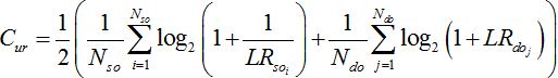
Where
 Number of same- and different-speaker comparisons, respectively;
 LRs determined for same- and different-speaker origins, respectively.
Low
values indicate that a FVC analysis system is providing some useful information (the lower the value, the more accurate the analysis, and vice versa).Tippett plot:
Applied Probability of Error (APE) plot:
=0), but in reality every system will have losses. The loss in  is typically divided into discrimination loss and calibration loss
  . corresponds to the lowest that can be achieved while preserving the discrimination power of the system. This corresponds to the area under the green APE curve which is also equal to the height of the green bar. can be obtained by subtracting from and corresponds to the area between the red and green APE curves. It is equal to height of the red bar. The combined height of the green and red bars gives the actual of the system.
Credible Interval (CI) as a measure of reliability/precision:
METHODOLOGY
Speech database and speech parameters
Speakers in this database were recorded on four separate occasions separated by one month intervals. During each recording session, each subject repeated three ‘sentences’ twice. The first two of these comprised a sequence of random digits, as follows: “zero one two three four five six seven eight nine†and “five zero six nine two eight one three seven fourâ€. The last sentence was a phonetically balanced sentence: “Joe took father’s green shoe bench outâ€. The speech files are sampled at 32 kHz and digitized into 16 bits. The vowel segments /aI/, /eI/ and /i/ have then been extracted from the words “nineâ€, “eight†and “threeâ€, respectively. The realization of different phonemes was manually located in the speech files using a combination of auditory and acoustic analysis. Audio editing programs, such as Goldwave [32] and Wave surfer [33], were used to assist in this process. Even though the database contains four different recording sessions, only three of them were used here. In summary, four tokens of three different vowels (two diphthongs and one monophthong) from three non-contemporaneous recordings were used in the following FVC experiments.
All speech samples were down-sampled to 8 kHz and stored into 16 bit PCM wav files to align with the input speech requirements of mobile phone speech codecs. Different types of noise at different SNR levels were added to the speech samples and these then coded under certain modes of operation in both the GSM and CDMA networks. MFCCs were then extracted from the vowel segments as follows. A Hamming window was applied to the whole vowel segment to remove edge effects, followed by taking its Discrete Fourier Transform (DFT). A set of 23 Mel-filter banks were then applied to the speech signal in the frequency domain. The average energy was estimated in each frequency band, followed by taking its logarithm. A Discrete Cosine Transform (DCT) was then applied, resulting in a total of 23 MFCCs
 [34].
[34].The 130 speakers chosen for this experiment were divided as follows: 44 speakers for the Background set, 43 speakers for the Development set and 43 speakers for the Testing set. Two same-speaker comparisons were obtained for each speaker in the Testing set by comparing their tokens from Session 1 with their tokens from Sessions 2 and 3. Similarly, three different-speaker comparisons were obtained for each speaker by comparing their tokens from Session 1 with all other speakers’ tokens from Sessions 1, 2 and 3. The Background set remained the same across all comparisons and included tokens from two recording sessions for each of the 44 Background speakers. The sole purpose of the Development set is to train the fusion system, the resulting weights of which are used to combine LRs calculated from individual vowels for every comparison in the testing set [35].
The mean values for each two same-speaker and three different-speaker LLRs were calculated and then a
value was calculated from those means. This will be referred to in this paper as Mean . The CI was calculated by finding the variation in each LR calculation (i.e., variation between two same-speaker and three different-speaker comparisons) using the non-parametric approach and then taking their average.Experimental procedure
and CI between two FVC analyses for each network. The first used clean speech processed by the codec under specific modes of operation. The second used speech that had been corrupted with different types of BN at different SNRs and then coded using the same modes of operation as for the clean speech.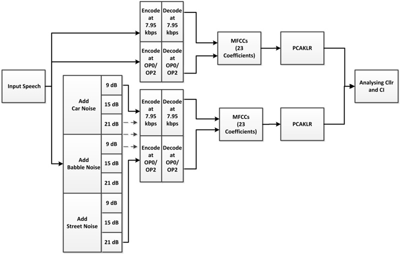 Figure 1: Block diagram of the experimental setup.
The three types of BN used in our experiments (car, babble, and street noise) were acquired from the Soundjay database [36]. Each of these was added to the speech files at three SNRs: 9, 15, and 21 dB, according to [37]. To reflect more realistic scenarios in these experiments, different sections of noise were added to the speech samples. Only matched conditions have been considered here, where the Background set contained coded speech at the same specific mode being investigated, but without BN. The rationale with this was to investigate the impact of BN in isolation to other factors that might likely cloud the results.
Given that the speech codecs used in the GSM and CDMA networks are different in their operational modes, the kinds of experiments required to encompass the totality of all possible transmission scenarios for each network are necessarily different. In the GSM network the AMR codec uses a speech coding technique called Code-Excited Linear Prediction (CELP). It can operate at one of eight source coding bit rates: 4.75, 5.15, 5.90, 6.70, 7.40, 7.95, 10.20 and 12.20 kbps [38]. Though the AMR codec can switch between bit rates every 40 ms [39], only the median bit rate, namely 7.95 kbps, has been used in our experiments. The rationale for this is that a bit rate of 7.95 kbps is likely to be used in the GSM network when channel conditions are average (i.e., neither too good nor too poor). The Background set was also coded at 7.95 kbps using clean speech.
In the CDMA network the EVRC codec can operate at three different modes of operation, called Anchor Operating Points (AOPs): OP0, OP1 and OP2, which are designed to change the speech coding bit rate in accordance with different channel and capacity conditions present in the network, producing high-, medium- and low-quality speech, respectively. Two sets of experiments have been conducted using CDMA-quality speech. The first used clean speech processed by the codec at modes OP0 and OP2. For the second, different kinds of BN, at various SNR levels, were added prior to processing them at either OP0 or OP2.
The rationale for conducting FVC experiments at two different AOPs is that OP0 incorporates a different set of coding algorithms to either OP1 or OP2. These latter two use a combination of Pitch Period Prototype (PPP) and CELP for coding vowels, whereas OP0 uses only CELP. The PPP algorithm exploits the fact that pitch patterns do not dramatically change from one frame to another. Thus, rather than transmitting pitch information for every speech frame, information from previous frames is used, while resolving any discontinues arising from phase misalignment [4,40]. As will be discussed in the next section, this repetition of pitch patterns can mask the effect of NS, which in turn improves the comparison results when low-quality speech coding is used, as would be the case for mode OP2. OP1 has not been investigated here because it essentially uses the same coding processes as OP2.
RESULTS AND DISCUSSION
Impact of the EVRC’s NS Process on the speech time waveform
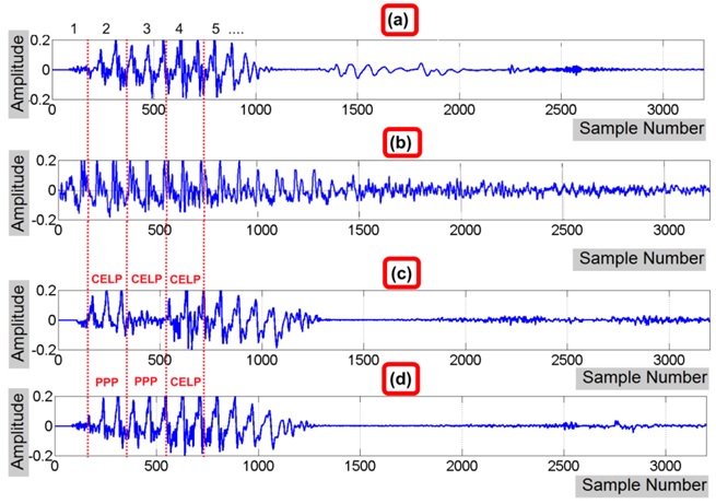 Figure 2: The impact of NS under different anchor operating points on a token of the word ‘eight’. The vertical dotted lines indicate frame boundaries. (a) Clean speech, (b) Clean speech with street noise added as SNR=6 dB, (c) Noisy speech coded using OP0, and (d) Noisy speech coded using OP2.
Examination of Figure 2 reveals that the EVRC has done a good job in reducing BN despite the high levels of added noise. However, speech signal characteristics have changed slightly as a result of the NS process. In the case of OP0 (Figure 2(c)) a large part of the original speech in Frame 3, together with the BN originally present there, have been removed. Interestingly, this was not the case for OP2, where Frame 3 remained intact after NS. Though this might cause some surprise, given that OP2 is expected to produce lower speech quality than OP0, it arises as a result of the use of PPP in OP1 and OP2, which exploits the fact that pitch contours do not significantly change over two or more consecutive frames. In light of this, one might expect a poorer performance of FVC when using high-quality coded speech (i.e., OP0) in the presence of high BN levels (i.e., low SNRs).
Impact of BN in the GSM network
| AMR Mode: | 7.95 kbps | ||
| Noise Type | SNR | Mean Cllr | CI |
| Car | 21dB | 0.128 | 1.538 |
| 15dB | 0.146 | 1.591 | |
| 9dB | 0.184 | 1.688 | |
| Babble | 21dB | 0.145 | 1.576 |
| 15dB | 0.162 | 1.587 | |
| 9dB | 0.193 | 1.801 | |
| Street | 21dB | 0.153 | 1.691 |
| 15dB | 0.160 | 1.616 | |
| 9dB | 0.180 | 1.542 | |
| No Noise | 0.128 | 1.620 | |
Table 1: Performance of FVC analysis in the GSM network with speech coded at 7.95 kbps using various types and levels of BN.
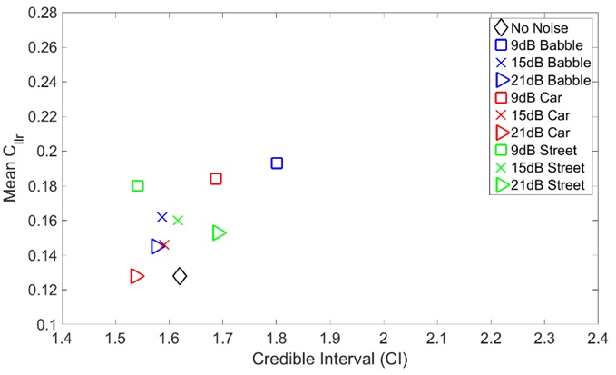 Figure 3: Mean vs CI in the GSM network for speech coded at 7.95 kbps with different types of noise added at different SNR levels.
It is clear from figure 3 that the accuracy of the FVC results generally gets worse in the presence of noise. The accuracy is worse when SNR is low across all three types of BN, with babble noise being the worst in this respect. Car noise tends to have almost no impact on accuracy at high SNR levels. Further, it can be seen from figure 3 that for a particular SNR level, different types of noise have resulted in a relatively similar accuracy for low SNR.
Some insight into why the accuracy gets worse in the presence of background noise in the GSM network can be gained by comparing the Tippett plot of figure 4 for clean-coded speech with that of figure 5 for speech corrupted with babble noise at 9dB SNR. The solid blue curve in this figure represents the same-speaker comparison results and the solid red curve the different-speaker comparisons. The dashed lines shown on the either side of the solid blue and red curves represent the variation found in a particular LR comparison result (i.e.,
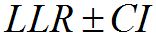 ).
).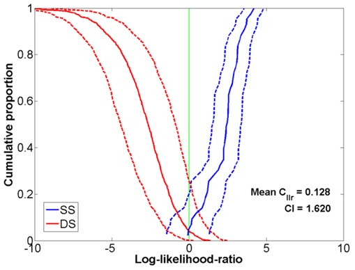 Figure 4: Tippett plot showing the FVC performance using clean speech coded at 7.95kbps in the GSM network.
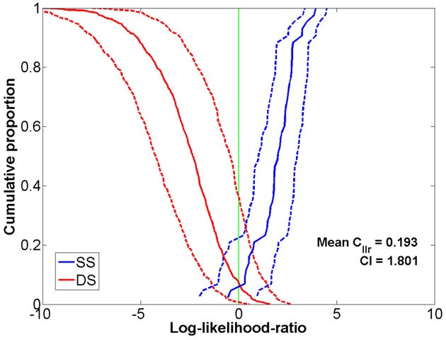 Figure 5: Tippett plot showing the FVC performance using speech in the GSM network corrupted by babble noise at 9 dB SNR and coded at 7.95 kbps., APE plots for the babble noise case are shown in figure 6.
 Figure 6: APE plot showing the FVC performance using speech in the GSM network corrupted by babble noise added at various SNR levels and coded at 7.95 kbps.
Firstly, in all cases including clean-coded speech, the
is dominated by discrimination loss . This is worse at lower SNR, which is an expected trend (i.e., speech parameters lose their discrimination power in the presence of large amounts of noise). In respect to calibration loss, differences between clean and noisy speech are very small, though the former has a slightly worse performance than the latter, especially at high SNR. The same trend is observed for the discrimination and calibration losses for the other types of noise as well.Impact of BN in the CDMA network
and CI. This is because the process of NS is expected to function more effectively under such SNR levels. The CI for both speech coding qualities improved for most of the BN experiments compared to the clean-coded speech experiments. This is an unexpected result and it is not clear at this stage why this is happening.| EVRC Mode: | OP0 | OP2 | |||
| Noise Type | SNR | Mean Cllr |
CI | Mean Cllr | CI |
| Car | 21dB | 0.149 | 1.655 | 0.146 | 1.608 |
| 15dB | 0.152 | 1.585 | 0.152 | 1.616 | |
| 9dB | 0.185 | 1.537 | 0.172 | 1.793 | |
| Babble | 21dB | 0.144 | 1.686 | 0.143 | 1.914 |
| 15dB | 0.146 | 2.262 | 0.128 | 2.071 | |
| 9dB | 0.265 | 1.503 | 0.190 | 2.306 | |
| Street | 21dB | 0.143 | 1.792 | 0.165 | 1.914 |
| 15dB | 0.169 | 1.645 | 0.167 | 1.714 | |
| 9dB | 0.247 | 1.658 | 0.209 | 1.825 | |
| No Noise | 0.117 | 1.891 | 0.116 | 1.953 | |
Table 2: FVC Performance in the CDMA network using speech coded at OP0 and OP2 under various BN conditions.
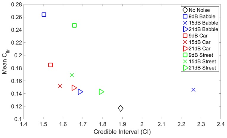 Figure 7: Mean
  vs CI for speech in the CDMA network coded at OP0 with different types of noise added at different SNR levels.
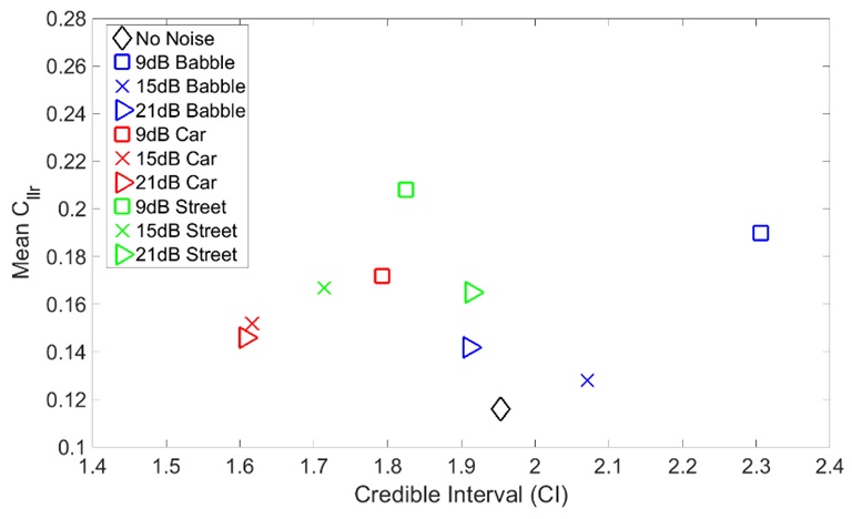 Figure 8: Mean vs CI for speech in the CDMA network coded at OP2 with different types of noise added at different SNR levels. decreases for the lower coding quality as compared to the higher coding quality. It should not be inferred from this, though, that the accuracy improves as the SNR decreases for low-quality coding (i.e., OP2), but rather that the accuracy for OP2 is better than OP0 at high BN levels. We conjecture that this behaviour is linked to the coding pattern for sequential frames used in OP2. Specifically, this coding pattern, together with high levels of BN, is likely to introduce slightly more variation between the speech samples of all speakers and thus increase between-session variations. This is evident in the elevated CI values of the OP2 results at low SNRs. In the case of OP0, the NS process subtracts BN from every speech frame without a mechanism, such as PPP, to mitigate this effect. This can result in samples that are more similar, but highly distorted, which affects the measurement of the speech parameters of interest. As a result, better CI and worse can be observed in this case. The situation reverses for these two coding qualities when BN levels are low (i.e., with SNRs above 15dB in this case), where the and CI values are better for OP0 than OP2, which is an expected behaviour. Again, this is a result of the NS process being able to function more effectively at higher SNRs.
In order to examine the BN impact with respect to the same- and different- speaker comparisons, Tippett plots have also been produced for all the experiments for babble noise. Tippett plots for the other types of BN have not been shown here as they are very similar to those for babble noise.
Figures 9 and 10 show Tippett plots for the FVC results using clean speech coded with OP0 and OP2, respectively. Figures 11 and 12 show the corresponding results for OP0 and OP2, respectively, for the case of babble noise at 9dB SNR. In the case of high BN levels, the addition of BN causes a significant increase in the proportion of both same- and different-speaker misclassifications and we conjecture that these are worse for high-quality speech coding for the reasons previously mentioned. As the SNR increases, it appears that only different-speaker comparisons are negatively impacted. The degree of this impact was almost the same for both coding qualities.
 Figure 9: Tippett plot showing the FVC performance using clean speech in the CDMA network coded at OP0.
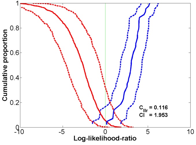 Figure 10: Tippett plot showing FVC performance using clean speech in the CDMA network coded at OP2.
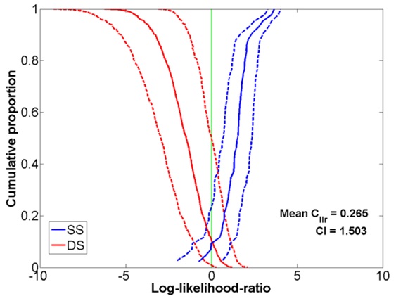 Figure 11: Tippett plot showing the FVC performance using speech in the CDMA network corrupted by babble noise at 9dB SNR and coded at OP0.
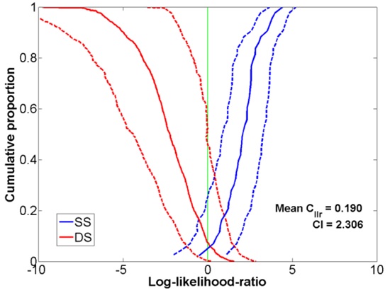 Figure 12: Tippett plot showing the FVC performance using speech in the CDMA network corrupted by babble noise at 9dB SNR and coded at OP2.
In order to analyze the losses in
, APE plots were produced for the babble noise experiments. Again these were found to be typical of the other types of noise and therefore their APE plots are not shown here. The APE plots in figures 13 and 14 correspond to the OP0 and OP2 experiments, respectively, using speech files corrupted with babble noise at various SNR levels. Analysis of these plots reveals that the degradation in is mainly attributable to a decrease in the discrimination performance of the speech parameters (i.e., ). The presence of high levels of BN combined with low-quality coded speech causes the discrimination loss to increase. The situation was even worse for the higher speech quality. The calibration performance for all the cases was found comparable, but it tends to be higher (i.e., worse) for higher-quality speech coding when SNR levels are low.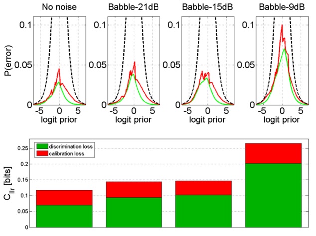 Figure 13: APE plot showing the FVC performance using speech corrupted by babble noise added at various SNR and coded at OP0.
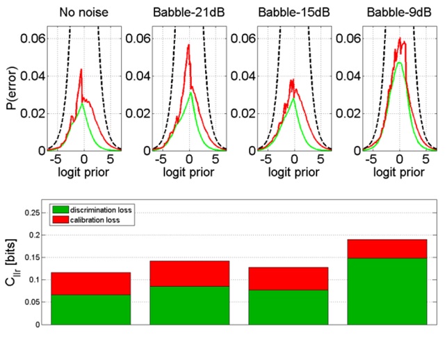 Figure 14: APE plot showing the FVC performance using speech corrupted by babble noise added at various SNR and coded at OP2.
CONCLUSION
In this paper we have presented the impact of BN on the strength of evidence associated with a FVC analysis when using speech processed by either the GSM or CDMA mobile phone networks. These two major phone technologies are fundamentally different in their design and in their ways of handling BN, so their impact on the results of a FVC is also different. Three different kinds of BN at different SNR levels have been considered in our experiments, namely babble, street and car noises.
As expected, for both networks the accuracy of the FVC results was found to be worse when using noisy speech compared to clean-coded speech. Further, the higher the BN levels the worse the accuracy. This is because the speech parameters used for comparison begin to lose their potential for discriminating between speakers at high BN levels, as is evidenced in the higher discrimination losses observed under such conditions. The CDMA network tends to have a greater impact than the GSM network on FVC accuracy under noisy speech scenarios. The situation is even worse when the CDMA network uses high-quality speech coding, which would be the case if a call was made from a low populated area. This is due to the fact that the low-quality speech coding modes, such as OP1 and OP2, can mask the impact of BN by repeating information from previous frames, whereas this mechanism does not occur for high-quality coding (i.e., OP0).
The reliability of the FVC analysis was not significantly impacted by the addition of BN for either of the networks. In fact, this aspect improved for most of the investigated scenarios with BN.
REFERENCES
- 3GPP2 (2013) Enhanced Variable Rate Codec, Speech Service Options 3, 68, 70, and 73 for Wideband Spread Spectrum Digital Systems. S0014-D, 3rd Generation Partnership Project 2 (3GPP2), USA.
- Punter S (2013) Southern Ontario Cell Phone Page. ARCX Inc., USA.
- 3GPP2 (2012) Minimum Performance Specification for the Enhanced Variable Rate Codec, Speech Service Options 3 and 68 for Wideband Spread Spectrum Digital Systems. S0018-B, 3rd Generation Partnership Project 2 (3GPP2), USA.
- Alzqhoul EAS, Nair BBT, Guillemin BJ (2014) An Alternative Approach for Investigating the Impact of Mobile Phone Technology on Speech International Conference on Signal Processing and Imaging Engineering. 2014 International Conference on Signal Processing and Imaging Engineering (ICSPIE’15), San Francisco, USA.
- Alzqhoul EA, Nair BB, Guillemin BJ (2012) Speech Handling Mechanisms of Mobile Phone Networks and Their Potential Impact on Forensic Voice Analysis. 14th Australasian International Conference on Speech Science and Technology, Sydney, Australia.
- Guillemin BJ, Watson C (2008) Impact of the GSM Mobile Phone Network on the Speech Signal-Some Preliminary Findings. International Journal of Speech Language and the Law 15: 193-218.
- Aitken CG, Lucy D (2004) Evaluation of trace evidence in the form of multivariate data. Journal of the Royal Statistical Society: Series C, Appl Statist 53: 109-122.
- Nair BBT, Alzqhoul E, Guillemin BJ (2014) Determination of likelihood ratios for forensic voice comparison using Principal Component Analysis. International Journal of Speech Language and the Law 21: 83-112.
- Reynolds DA, Quatieri TF, Dunn RB (2000) Speaker verification using adapted Gaussian mixture models. Digital signal processing 10: 19-41.
- Kim W, Hansen JH (2009) Feature compensation in the cepstral domain employing model combination. Speech Communication 51: 83-96.
- Milner B, Darch J, Vaseghi S (2008) Applying noise compensation methods to robustly predict acoustic speech features from MFCC vectors in noise. Acoustics, Speech and Signal Processing 2008, ICASSP 2008, IEEE International Conference on 2008, Las Vegas, NV.
- Pelecanos J, Sridharan S (2001) Feature warping for robust speaker verification.
- 3GPP (2013) Mandatory Speech Codec speech processing functions; Adaptive Multi-Rate (AMR) speech codec; Error concealment of lost frames. 3GPP, TS 26.091 3rd Generation Partnership Project; Technical Specification Group Services and System Aspects.
- 3GPP2 (2013) Enhanced Variable Rate Codec, Speech Service Options 3, 68, and 70 for Wideband Spread Spectrum Digital Systems. 3GPP2-EVRC, 3rd Generation Partnership Project 2 (3GPP2), USA.
- Isabelle SH, Solana Technology Dev Corp. (2000) Noise suppression for low bitrate speech coder. WO2000017859 A8.
- Lee S-M, Y-J Kim, Samsung Electronics Co., Ltd. (2002) Method for eliminating annoying noises of enhanced variable rate codec (EVRC) during error packet processing. US6385578 B1.
- Proakis JG, Manolakis DG (1996) Digital signal processing: principles, algorithms, and application. (3rdedn), Prentice-Hall International, New Jersey, USA.
- Gonzalez-Rodriguez J, Ros P, Ramos D, Toledano DT, Orlega-Garcia J (2007) Emulating DNA: Rigorous quantification of evidential weight in transparent and testable forensic speaker recognition. IEEE Transactions on Audio, Speech, and language processing 15: 2104-2115.
- Rose P (2004) Forensic speaker identification. CRC Press, USA.
- Morrison GS (2010) Forensic voice comparison. In: Freckelton I, Selby H (eds.). Expert Evidence (chapter 99), Thomson Reuters, Sydney, Australia.
- Morrison GS (2009) Forensic voice comparison and the paradigm shift. Sci Justice 49: 298-308.
- Saks MJ, Koehler JJ (2005) The coming paradigm shift in forensic identification science. Science 309: 892-895.
- Morrison GS (2011) Measuring the validity and reliability of forensic likelihood-ratio systems. Sci Justice 51: 91-98.
- Rose P (2003) The technical comparison of forensic voice samples. In: Selby H, Freckelton I (eds.). Expert Evidence (chapter 99), Thompson Lawbook Co, Sydney, Australia.
- Meuwly D, Drygajlo A (2001) Forensic speaker recognition based on a Bayesian framework and Gaussian Mixture Modelling (GMM). The Speaker Recognition Workshop, 2001: A Speaker Odyssey, Crete, Greece.
- Brümmer N, Burget L, Cernocky JH, Glembek O, Grezl F (2006) Fusion of heterogeneous speaker recognition systems in the STBU submission for the NIST speaker recognition evaluation 2006. IEEE Transactions on Audio, Speech, and Language Processing 15: 2072-2084.
- Brümmer N, J du Preez (2006) Application-independent evaluation of speaker detection. Comput Speech Lang 20: 230-275.
- Morrison GS, Thiruvaran T, Epps J (2010) Estimating the precision of the likelihood-ratio output of a forensic-voice-comparison system. The Speaker and Language Recognition Workshop, Odyssey 2010, Czech Republic.
- Morrison GS, Zhang C, Rose P (2011) An empirical estimate of the precision of likelihood ratios from a forensic-voice-comparison system. Forensic Sci Int 208: 59-65.
- Messer K, Matas J, Kittler J (1999) XM2VTSDB: The extended M2VTS database. Second international conference on audio and video-based biometric person authentication. Citeseer, Washington, DC, USA.
- Morrison GS, Ochoa F, Thiruvaran T (2012) Database selection for forensic voice comparison. The Speaker and Language Recognition Workshop, Odyssey 2012, Singapore.
- Goldwave Inc. (2013) Gold Wave digital audio editor. Goldwave Inc., St. John’s, NL, Canada.
- Centre for Speech Technology (CTT) (2013) Wave Surfer. Centre for Speech Technology, KTH, Stockholm, Sweden.
- Rabiner LR, Schafer RW (2010) Theory and application of digital speech processing. (1stedn), Prentice Hall, Pearson Education, New Jersey, USA.
- Ramos-Castro D, Gonzalez-Rodriguez J, Ortega-Garcia J (2006) Likelihood ratio calibration in a transparent and testable forensic speaker recognition framework. In: Speaker and Language Recognition Workshop, 2006. IEEE, Odyssey.
- Soundjay (2013) Soundjay Sound Effects website. Soundjay, Finland.
- ITU-T (2013) Objective measurement of active speech level ITU-T Recommendation P-56. International Telecommunication Union (ITU), USA.
- 3GPP (2012) Technical Specification Group Services and System Aspects; Mandatory speech CODEC speech processing functions; AMR speech CODEC; General description. TS 26.071 V11.0, 3rd Generation Partnership Project, USA.
- 3GPP (2013) Technical Specification Group GSM/EDGE Radio Access Network; Link adaptation. TS 45.009, 3rd Generation Partnership Project, USA.
- Alzqhoul EA, Nair BB, Guillemin BJ (2012) Speech Handling Mechanisms of Mobile Phone Networks and Their Potential Impact on Forensic Voice Analysis. In: SST, 14th Australasian International Conference on Speech Science and Technology Sydney, Australia.
- Alzqhoul EA, Nair BB, Guillemin BJ (2015) Impact of dynamic rate coding aspects of mobile phone networks on forensic voice comparison. Sci Justice 55: 363-374.
Citation: Alzqhoul EAS, Nair BBT, Guillemin BJ (2016) Impact of Background Noise in Mobile Phone Networks on Forensic Voice Comparison. J Forensic Leg Investig Sci 2: 007.
Copyright: © 2016 Esam AS Alzqhoul, et al. This is an open-access article distributed under the terms of the Creative Commons Attribution License, which permits unrestricted use, distribution, and reproduction in any medium, provided the original author and source are credited.